Multiple Linear Regression using Python

• by administrator
• 15 March, 2022

This article was published as a part of the Data Science Blogathon.

Table of Contents

Introduction

Working with Dataset

Define X and Y

Perform OneHotEncoding

Change columns using Column Transformer

Split the dataset into train set and test set

Train the model

Predict the test Results

Evaluate the model

Plot the Results

Predicted Values

Introduction

In this article, we will be dealing with multi-linear regression and we will take a dataset that contains information about 50 startups. Features include R&D Spend, Administration, Marketing Spend, State, and finally Profit. Here we have to build the machine learning model to predict the profit of the startups.

Let’s get started.

Source: https://encrypted-tbn0.gstatic.com/images?q=tbn:ANd9GcRyRUO-bCMGcQAG7G-KFtg8J0bFOO0vRnUdQQ&usqp=CAU

Multiple linear regression is one of the most important machine learning algorithms where we provide multiple independent variables for a single dependent outcome variable. Whereas for linear regression we just provide one independent variable as input.

Working with Dataset

Let’s start by importing some libraries.

import numpy as np
import pandas as pd
from sklearn.model_selection import train_test_split
from sklearn.linear_model import LinearRegression
from sklearn.metrics import r2_score
import matplotlib.pyplot as plt
import seaborn as sns
import warnings
warnings.filterwarnings("ignore")

Import train_test_split to split the dataset into training and testing datasets. And LinearRegression is the model on which we have to work. Import this model from scikit learn library. r2_score is to find the accuracy of the model. Matplotlib and seaborn are used for visualizations. Finally import warnings and set it to ignore so that it will ignore all the warnings that we will come throughout.

Here is the link for the dataset. Download it and import it by passing the path of the dataset file into read_csv().

#import dataset
startup_df=pd.read_csv(r'C:UsersAdminDownloadsstartups_dataset.csv')

Let us view our data frame.

startup_df

Source: Author

Source: Author

Source: Author

View the shape of the data frame.

shape=startup_df.shape
print("Dataset contains {} rows and {} columns".format(shape[0],shape[1]))

The dataset contains 50 rows and 5 columns

View all the columns in the data frame.

startup_df.columns

Source: Author

Data frame contains R&D Spend, Administration, Marketing Spend, State, and Profit.

View the statistical description of the dataset which includes the total count of each column, mean of all values, standard deviation, minimum, maximum values, and 25th, 50th, 75th per cent values of the dataset.

#Statistical Details of the dataset
startup_df.describe()

Source: Author

Define X and Y

This is like extracting dependent and independent variables.

We have to define x and y for the model. x and y are input and output features of the dataset. So taking x features as input values that are independent, our model will predict the outcome which is y that are dependent.

x=startup_df.iloc[:,:4]
y=startup_df.iloc[:,4]

Perform One-Hot Encoding

Source: https://encrypted-tbn0.gstatic.com/images?q=tbn:ANd9GcRvSKvzOSO1qozi7gdygfZkDvvdNW7ocy3PLw&usqp=CAU

We use one-hot encoding when there are categorical values in our dataset. Here for us, there is a state column that is categorical so we have to use one-hot encoding to convert them.

So import OneHotEncoder from scikit learn library.

from sklearn.preprocessing import OneHotEncoder
ohe=OneHotEncoder(sparse=False)
x=ohe.fit_transform(startup_df[['State']])

View x.

x

array([[0., 0., 1.],
[1., 0., 0.],
[0., 1., 0.],
[0., 0., 1.],
[0., 1., 0.],
[0., 0., 1.],
[1., 0., 0.],
[0., 1., 0.],
[0., 0., 1.],
[1., 0., 0.],
[0., 1., 0.],
[1., 0., 0.],
[0., 1., 0.],
[1., 0., 0.],
[0., 1., 0.],
[0., 0., 1.],
[1., 0., 0.],
[0., 0., 1.],
[0., 1., 0.],
[0., 0., 1.],
[1., 0., 0.],
[0., 0., 1.],
[0., 1., 0.],
[0., 1., 0.],
[0., 0., 1.],
[1., 0., 0.],
[0., 1., 0.],
[0., 0., 1.],
[0., 1., 0.],
[0., 0., 1.],
[0., 1., 0.],
[0., 0., 1.],
[1., 0., 0.],
[0., 1., 0.],
[1., 0., 0.],
[0., 0., 1.],
[0., 1., 0.],
[1., 0., 0.],
[0., 0., 1.],
[1., 0., 0.],
[1., 0., 0.],
[0., 1., 0.],
[1., 0., 0.],
[0., 0., 1.],
[1., 0., 0.],
[0., 0., 1.],
[0., 1., 0.],
[1., 0., 0.],
[0., 0., 1.],
[1., 0., 0.]])

It will give an array like this. let us see what are those three categories.

ohe.categories_

[array([‘California’, ‘Florida’, ‘New York’], dtype=object)]

Here [0., 0., 1.] indicates NewYork, [0., 1., 0.] indicates Florida  and [1., 0., 0.] indicates California.

Change Columns using Column Transformer

For this import make_column_transformer from scikit learn library. and pass the column that we want to transfer.

from sklearn.compose import make_column_transformer

col_trans=make_column_transformer(
    (OneHotEncoder(handle_unknown='ignore'),['State']),
    remainder='passthrough')

x=col_trans.fit_transform(x)

Now view x

It will look like this.

Source: Author

Split the Dataset into Train Set and Test Set

Now split your dataset into two parts in which 80% of the dataset will go to the training set and 20% of the dataset will go to the testing set. Actually, you can divide it as per your wish by setting the value into test_size.

x_train,x_test,y_train,y_test=train_test_split(x,y,test_size=0.2,random_state=0)

View the shapes of splitter data.

#shapes of splitted data
print("X_train:",x_train.shape)
print("X_test:",x_test.shape)
print("Y_train:",y_train.shape)
print("Y_test:",y_test.shape)

X_train: (40, 6)
X_test: (10, 6)
Y_train: (40,)
Y_test: (10,)

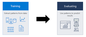
Train the Model

Source: https://docs.microsoft.com/en-us/windows/ai/images/winml-model-flow.png

To train the model we have to import the LinearRegression model which we have already done at the beginning. Use the fit method and pass the training sets into it to train the model.

linreg=LinearRegression()
linreg.fit(x_train,y_train)

Predict the Test Results

Predict the results using predict method and pass the independent variables of the testing data set into it and view them. It will give the array with all the values in it.

y_pred=linreg.predict(x_test)
y_pred

Source: Author

Evaluate the Model

We have different metrics to find the accuracy score of the model and here we use r2_score to evaluate our model and find its accuracy.

Accuracy=r2_score(y_test,y_pred)*100
print(" Accuracy of the model is %.2f" %Accuracy)

The accuracy of the model is 93.47.

Plot the Results

We will plot the scatter plot between actual values and predicted values. Use xlabel to label the x-axis and use ylabel to label the y-axis.

plt.scatter(y_test,y_pred);
plt.xlabel('Actual');
plt.ylabel('Predicted');

Source: Author

Regression plot of our model.

A regression plot is very useful to understand the linear relationship between two parameters. It creates a regression line in between those parameters and a scatter plot of data points was plotted.

sns.regplot(x=y_test,y=y_pred,ci=None,color ='red');

Source: Author

Predicted Values

Let us create a new data frame that contains actual values, predicted values, and differences between them so that we will understand how near the model predicts its actual value.

pred_df=pd.DataFrame({'Actual Value':y_test,'Predicted Value':y_pred,'Difference':y_test-y_pred})

View the data frame

pred_df

Source: Author

Here we can see the difference between Actual values and predicted values which are not very high. When values are in the range of lakhs, then the difference in thousands is not much.
We have already seen that the accuracy of this model is about 93 per cent

Conclusion

In this article, we have created a new linear regression model and we learned how to perform one-hot encoding and where to perform it. We have used column transformer and finally trained the model, predicted the results, evaluated the model using r2_score metrics, plotted the results.

Hope you guys found it useful.

Read more articles on our website. Click here.

Connect with me on LinkedIn: https://www.linkedin.com/in/amrutha-k-6335231a6vl/

The media shown in this article is not owned by Analytics Vidhya and are used at the Author’s discretion. 

Size: Unknown Price: Free Author: Amrutha K Data source: https://www.analyticsvidhya.com/