Machine Learning for Stock Market Prediction with Step-by-Step Implementation
- by user1
- 20 March, 2022
This article was published as a part of the Data Science Blogathon
Introduction to Stock Market Prediction
Stock market prediction and analysis are some of the most difficult jobs to complete. There are numerous causes for this, including market volatility and a variety of other dependent and independent variables that influence the value of a certain stock in the market. These variables make it extremely difficult for any stock market expert to anticipate the rise and fall of the market with great precision.
However, with the introduction of Machine Learning and its strong algorithms, the most recent market research and Stock Market Prediction advancements have begun to include such approaches in analyzing stock market data.
In summary, Machine Learning Algorithms are widely utilized by many organizations in Stock market prediction. This article will walk through a simple implementation of analyzing and forecasting the stock prices of a Popular Worldwide Online Retail Store in Python using various Machine Learning Algorithms.
.png)
Image 1
Problem statement for Stock Market Prediction
Let us see the data on which we will be working before we begin implementing the software to anticipate stock market values. In this section, we will examine the stock price of Microsoft Corporation (MSFT) as reported by the National Association of Securities Dealers Automated Quotations (NASDAQ). The stock price data will be supplied as a Comma Separated File (.csv), that may be opened and analyzed in Excel or a Spreadsheet.
MSFT’s stocks are listed on NASDAQ and their value is updated every working day of the stock market. It should be noted that the market does not allow trading on Saturdays and Sundays, therefore there is a gap between the two dates. The Opening Value of the stock, the Highest and Lowest values of that stock on the same days, as well as the Closing Value at the end of the day, are all indicated for each date.
The Adjusted Close Value reflects the stock’s value after dividends have been declared (too technical!). Furthermore, the total volume of the stocks in the market is provided, With this information, it is up to the job of a Machine Learning/Data Scientist to look at the data and develop different algorithms that may extract patterns from the historical data of the Microsoft Corporation stock.
The long short term memory
We will use the Long Short-Term Memory(LSTM) method to create a Machine Learning model to forecast Microsoft Corporation stock values. They are used to make minor changes to the information by multiplying and adding. Long-term memory (LSTM) is a deep learning artificial recurrent neural network (RNN) architecture.
Unlike traditional feed-forward neural networks, LSTM has feedback connections. It can handle single data points (such as pictures) as well as full data sequences (such as speech or video).
Program Implementation
We will now go to the section where we will utilize Machine Learning in Python to estimate the stock value using the LSTM.
Importing the Libraries
As we all know, the first step is to import the libraries required to preprocess Microsoft Corporation stock data and the other libraries required for constructing and visualizing the LSTM model outputs. We’ll be using the Keras library from the TensorFlow framework for this. All modules are imported from the Keras library.
#Importing the Libraries
import pandas as PD
import NumPy as np
%matplotlib inline
import matplotlib. pyplot as plt
import matplotlib
from sklearn. Preprocessing import MinMaxScaler
from Keras. layers import LSTM, Dense, Dropout
from sklearn.model_selection import TimeSeriesSplit
from sklearn.metrics import mean_squared_error, r2_score
import matplotlib. dates as mandates
from sklearn. Preprocessing import MinMaxScaler
from sklearn import linear_model
from Keras. Models import Sequential
from Keras. Layers import Dense
import Keras. Backend as K
from Keras. Callbacks import EarlyStopping
from Keras. Optimisers import Adam
from Keras. Models import load_model
from Keras. Layers import LSTM
from Keras. utils.vis_utils import plot_model
Getting to Visualising the Stock Market Prediction Data
Using the Pandas Data Reader library, we will upload the stock data from the local system as a Comma Separated Value (.csv) file and save it to a pandas DataFrame. Finally, we will examine the data.
#Get the Dataset
df=pd.read_csv(“MicrosoftStockData.csv”,na_values=[‘null’],index_col=’Date’,parse_dates=True,infer_datetime_format=True)
df.head()
Check for Null Values by printing the DataFrame Shape
In this step, firstly we will print the structure of the dataset. We check for null values in the data frame to ensure that there are none. The existence of null values in the dataset causes issues during training since they function as outliers, creating a wide variance in the training process.
#Print the shape of Dataframe  and Check for Null Values
print(“Dataframe Shape: “, df. shape)
print(“Null Value Present: “, df.IsNull().values.any())
Output:
>> Dataframe Shape: (7334, 6)
>>Null Value Present: False
| Date | Open | High | Low | Close | Adj Close | Volume |
| 1990-01-02 | 0.605903 | 0.616319 | 0.598090 | 0.616319 | 0.447268 | 53033600 |
| 1990-01-03 | 0.621528 | 0.626736 | 0.614583 | 0.619792 | 0.449788 | 113772800 |
| 1990-01-04 | 0.619792 | 0.638889 | 0.616319 | 0.638021 | 0.463017 | 125740800 |
| 1990-01-05 | 0.635417 | 0.638889 | 0.621528 | 0.622396 | 0.451678 | 69564800 |
| 1990-01-08 | 0.621528 | 0.631944 | 0.614583 | 0.631944 | 0.458607 | 58982400 |
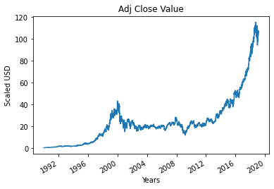
Step 4 – Plot of the True Adjusted Close Value
The Adjusted Close Value is the final output value that will be forecasted using the Machine Learning model. This figure indicates the stock’s closing price on that particular day of stock market trading.
#Plot the True Adj Close Value
df[‘Adj Close’].plot()

Setting the Target Variable and Selecting the Features
The output column is then assigned to the target variable in the following step. It is the adjusted relative value of the Microsoft Stock in this situation. Furthermore, we pick the features that serve as the independent variable to the target variable (dependent variable). We choose four characteristics to account for training purposes:
- Open
- High
- Low
- Volume
#Set Target Variable
output_var = PD.DataFrame(df[‘Adj Close’])
#Selecting the Features
features = [‘Open’, ‘High’, ‘Low’, ‘Volume’]
Scaling
To decrease the computational cost of the data in the table, we will scale the stock values to values between 0 and 1. As a result, all of the data in large numbers is reduced, and therefore memory consumption is decreased. Also, because the data is not spread out in huge values, we can achieve greater precision by scaling down. To perform this we will be using the MinMaxScaler class of the sci-kit-learn library.
#Scaling
scaler = MinMaxScaler()
feature_transform = scaler.fit_transform(df[features])
feature_transform= pd.DataFrame(columns=features, data=feature_transform, index=df.index)
feature_transform.head()
| Date | Open | High | Low | Volume |
| 1990-01-02 | 0.000129 | 0.000105 | 0.000129 | 0.064837 |
| 1990-01-03 | 0.000265 | 0.000195 | 0.000273 | 0.144673 |
| 1990-01-04 | 0.000249 | 0.000300 | 0.000288 | 0.160404 |
| 1990-01-05 | 0.000386 | 0.000300 | 0.000334 | 0.086566 |
| 1990-01-08 | 0.000265 | 0.000240 | 0.000273 | 0.072656 |
As shown in the above table, the values of the feature variables are scaled down to lower values when compared to the real values given above.
Creating a Training Set and a Test Set for Stock Market Prediction
We have to divide the entire dataset into training and test sets before feeding it into the training model. The Machine Learning LSTM model will be trained on the data in the training set and tested for accuracy and backpropagation on the test set.
The sci-kit-learn library’s TimeSeriesSplit class will be used for this. We set the number of splits to 10, indicating that 10% of the data will be used as the test set and 90% of the data would be used to train the LSTM model. The advantage of utilising this Time Series split is that the split time series data samples are examined at regular time intervals.
#Splitting to Training set and Test set
timesplit= TimeSeriesSplit(n_splits=10)
for train_index, test_index in timesplit.split(feature_transform):
        X_train, X_test = feature_transform[:len(train_index)], feature_transform[len(train_index): (len(train_index)+len(test_index))]
        y_train, y_test = output_var[:len(train_index)].values.ravel(), output_var[len(train_index): (len(train_index)+len(test_index))].values.ravel()
Data Processing For LSTM
Once the training and test sets are finalized, we will input the data into the LSTM model. Before we can do that, we must transform the training and test set data into a format that the LSTM model can interpret. As the LSTM needs that the data to be provided in the 3D form, we first transform the training and test data to NumPy arrays and then restructure them to match into the format (Number of Samples, 1, Number of Features). Now, 6667 are the number of samples in the training set, which is 90% of 7334, and the number of features is 4, therefore the training set is reshaped to reflect this (6667, 1, 4). Likewise, the test set is reshaped.
#Process the data for LSTM
trainX =np.array(X_train)
testX =np.array(X_test)
X_train = trainX.reshape(X_train.shape[0], 1, X_train.shape[1])
X_test = testX.reshape(X_test.shape[0], 1, X_test.shape[1])
Building the LSTM Model for Stock Market Prediction
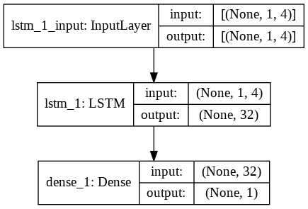
Finally, we arrive at the point when we will construct the LSTM Model. In this step, we’ll build a Sequential Keras model with one LSTM layer. The LSTM layer has 32 units and is followed by one Dense Layer of one neuron.
We compile the model using Adam Optimizer and the Mean Squared Error as the loss function. For an LSTM model, this is the most preferred combination. The model is plotted and presented below.
#Building the LSTM Model
lstm = Sequential()
lstm.add(LSTM(32, input_shape=(1, trainX.shape[1]), activation=’relu’, return_sequences=False))
lstm.add(Dense(1))
lstm.compile(loss=’mean_squared_error’, optimizer=’adam’)
plot_model(lstm, show_shapes=True, show_layer_names=True)

Training the Stock Market Prediction Model
Finally, we use the fit function to train the LSTM model created above on the training data for 100 epochs with a batch size of 8.
#Model Training
history=lstm.fit(X_train, y_train, epochs=100, batch_size=8, verbose=1, shuffle=False)
Eросh  1/100
834/834  [==============================]  –  3s  2ms/steр  –  lоss:  67.1211
Eросh  2/100
834/834  [==============================]  –  1s  2ms/steр  –  lоss:  70.4911
Eросh  3/100
834/834  [==============================]  –  1s  2ms/steр  –  lоss:  48.8155
Eросh  4/100
834/834  [==============================]  –  1s  2ms/steр  –  lоss:  21.5447
Eросh  5/100
834/834  [==============================]  –  1s  2ms/steр  –  lоss:  6.1709
Eросh  6/100
834/834  [==============================]  –  1s  2ms/steр  –  lоss:  1.8726
Eросh  7/100
834/834  [==============================]  –  1s  2ms/steр  –  lоss:  0.9380
Eросh  8/100
834/834  [==============================]  –  2s  2ms/steр  –  lоss:  0.6566
Eросh  9/100
834/834  [==============================]  –  1s  2ms/steр  –  lоss:  0.5369
Eросh  10/100
834/834  [==============================]  –  2s  2ms/steр  –  lоss:  0.4761
.
.
.
.
Eросh  95/100
834/834  [==============================]  –  1s  2ms/steр  –  lоss:  0.4542
Eросh  96/100
834/834  [==============================]  –  2s  2ms/steр  –  lоss:  0.4553
Eросh  97/100
834/834  [==============================]  –  1s  2ms/steр  –  lоss:  0.4565
Eросh  98/100
834/834  [==============================]  –  1s  2ms/steр  –  lоss:  0.4576
Eросh  99/100
834/834  [==============================]  –  1s  2ms/steр  –  lоss:  0.4588
Eросh  100/100
834/834  [==============================]  –  1s  2ms/steр  –  lоss:  0.4599
Finally, we can observe that the loss value has dropped exponentially over time over the 100-epoch training procedure, reaching a value of 0.4599.
LSTM Prediction
Now that we have our model ready, we can use it to forecast the Adjacent Close Value of the Microsoft stock by using a model trained using the LSTM network on the test set. This is accomplished by employing the simple predict function on the LSTM model that has been created.
#LSTM Prediction
y_pred= lstm.predict(X_test)
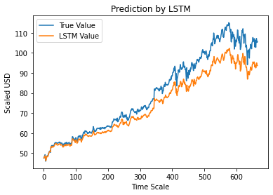
Comparing Predicted vs True Adjusted Close Value – LSTM
Finally, now that we’ve projected the values for the test set, we can display the graph to compare both Adj Close’s true values and Adj Close’s predicted value using the LSTM Machine Learning model.
#Predicted vs True Adj Close Value – LSTM
plt.plot(y_test, label=’True Value’)
plt.plot(y_pred, label=’LSTM Value’)
plt.title(“Prediction by LSTM”)
plt.xlabel(‘Time Scale’)
plt.ylabel(‘Scaled USD’)
plt.legend()
plt.show()

The graph above demonstrates that the extremely basic single LSTM network model created above detects some patterns. We may get a more accurate depiction of every specific company’s stock value by fine-tuning many parameters and adding more LSTM layers to the model.
Conclusion
However, with the introduction of Machine Learning and its strong algorithms, the most recent market research and Stock Market Prediction advancements have begun to include such approaches in analyzing stock market data. The Opening Value of the stock, the Highest and Lowest values of that stock on the same days, as well as the Closing Value at the end of the day, are all indicated for each date. Furthermore, the total volume of the stocks in the market is provided, With this information, it is up to the job of a Machine LearningData Scientist to look at the data and develop different algorithms that may help in finding appropriate stocks values.
Predicting the stock market was a time-consuming and laborious procedure a few years or even a decade ago. However, with the application of machine learning for stock market forecasts, the procedure has become much simpler. Machine learning not only saves time and resources but also outperforms people in terms of performance. it will always prefer to use a trained computer algorithm since it will advise you based only on facts, numbers, and data and will not factor in emotions or prejudice.
Image Source:
- Image 1: https://www.moneycontrol.com/news/photos/business/stocks/buzzing-stocks-tcs-nazara-technologies-ril-and-other-stocks-in-news-today-7566571.html
The media shown in this article are not owned by Analytics Vidhya and are used at the Author’s discretion.
Size: Unknown Price: Free Author: Prashant Sharma Data source: https://www.analyticsvidhya.com/