Guide for building an End-to-End Logistic Regression Model
- by user1
- 20 March, 2022
This article was published as a part of the Data Science Blogathon
In this blog, we’ll go over everything you need to know about Logistic Regression to get started and build a model in Python. If you’re new to machine learning and have never built a model before, don’t worry; after reading this, I’m confident you’ll be able to do so.
For those who are new to this, let’s start with a basic understanding of machine learning before moving on to Logistic Regression.
What is Machine Learning?
In simple terms, the Machine learning model uses algorithms in which the machine learns from the data just like humans learn from their experiences. Machine learning allows computers to find hidden insights without being explicitly programmed.
Types of Machine Learning algorithms
Based on the output type and task done, machine learning models are classified into the following types
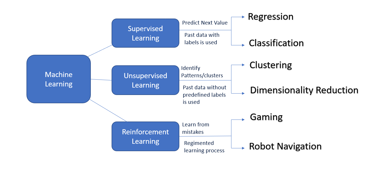
Logistic Regression falls under the Supervised Learning type. Let’s learn more about it.
Supervised Learning
It’s a type of Machine Learning that uses labelled data from the past. Models are trained using already labelled samples.
Example: You have past data of the football premier league and based on that data and previous match results you predict which team will win the next game.
Supervised learning is further divided into two types-
- Regression – target/output variable is continuous.
- Classification – target/output variable is categorical.
Logistic Regression is a Classification model. It helps to make predictions where the output variable is categorical. With this let’s understand Logistic Regression in detail.
What is Logistic Regression?
As previously stated, Logistic Regression is used to solve classification problems. Models are trained on historical labelled datasets and aim to predict which category new observations will belong to.
Below are few examples of binary classification problems which can be solved using logistic regression-
- The probability of a political candidate winning or losing the next election.
- Whether a machine in manufacturing will stop running in a few days or not.
- Filtering email as spam or not spam.
Logistic regression is well suited when we need to predict a binary answer (only 2 possible values like yes or no).
The term logistic regression comes from “Logistic Function,” which is also known as “Sigmoid Function”. Let us learn more about it.
Logistic/Sigmoid Function
The sigmoid function, commonly known as the logistic function, predicts the likelihood of a binary outcome occurring. The function takes any value and converts it to a number between 0 and 1. The Sigmoid Function is a machine learning activation function that is used to introduce non-linearity to a machine learning model.
The formula of Logistic Function is:
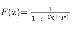
When we plot the above equation, we get S shape curve like below.
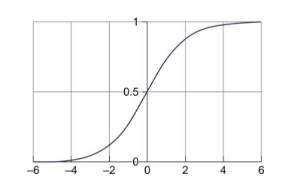
The key point from the above graph is that no matter what value of x we use in the logistic or sigmoid function, the output along the vertical axis will always be between 0 and 1.
When the result of the sigmoid function is greater than 0.5, we classify the label as class 1 or positive class; if it’s less than 0.5, we can classify it as a negative class or 0.
In Logistic Regression, iterative optimization algorithms like Gradient Descent or probabilistic methods like Maximum Likelihood are used to get the “best fit” S curve.
Let’s understand the mathematics behind the sigmoid function.
Logistic regression is derived from Linear regression bypassing its output value to the sigmoid function and the equation for the Linear Regression is –

In Linear Regression we try to find the best-fit line by changing m and c values from the above equation and y (output) can take any values from -infinity to +infinity. But, Logistic regression predicts the probability of outcome which can be between 0 to 1. So, to convert those values between 0 to 1 we use the sigmoid function.

after getting our output value we need to see how our model works, for that, we need to calculate the loss function. The loss function tells us how much our predicted output differ from the actual output. A good model should have less loss value. Let’s see how to calculate the loss function.
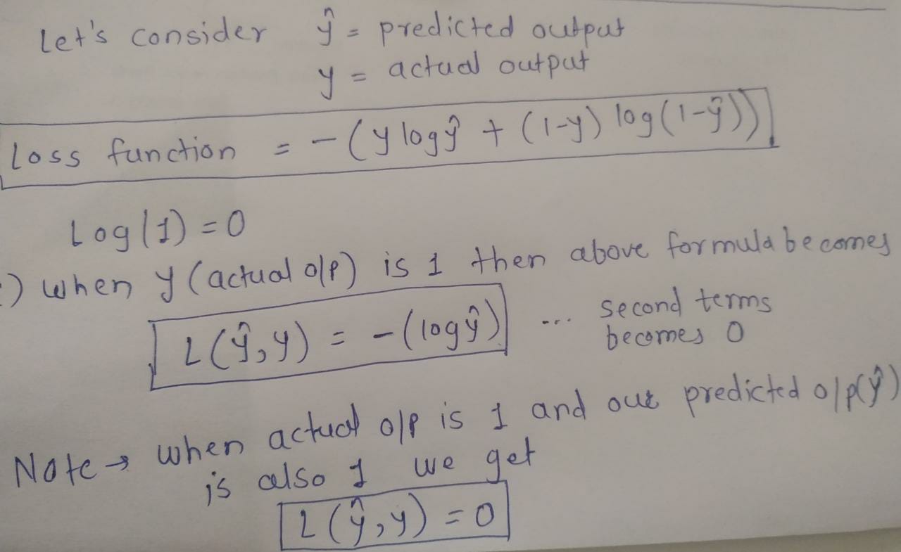
When y=1, the predicted y value should be close to 1 to reduce the loss. Now Let’s see when our actual output value is 0.
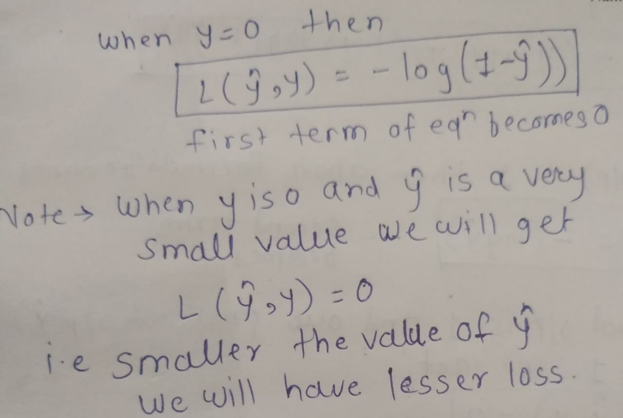
When y=0, the predicted y value should be close to 0 to reduce the loss.
Let’s move on to the implementation of the Logistic Regression model now that we’ve covered the basics.
Step by step implementation of Logistic Regression Model in Python
Based on parameters in the dataset, we will build a Logistic Regression model in Python to predict whether an employee will be promoted or not.
For everyone, promotion or appraisal cycles are the most exciting times of the year. Final promotions are only disclosed after employees have been evaluated on a variety of criteria, which causes a delay in transitioning to new responsibilities. We will build a Machine Learning model to predict who is qualified for promotion to speed up the process.
You can get more understanding of the problem statement and download the dataset from Supervised learning.
Importing Libraries
We’ll begin by loading the necessary libraries for creating a Logistic Regression model.
import numpy as np
import pandas as pd
#Libraries for data visualization
import matplotlib.pyplot as plt
import seaborn as sns
#We will use sklearn for building logistic regression model
from sklearn.linear_model import LogisticRegression
Loading Dataset
We’ll
use the HR Analytics dataset from the link above. We’ll start by loading the
dataset from the downloaded CSV file with the code below.
# Loading dataset from CSV file
data= pd.read_csv("train_LZdllcl.csv",sep=",")
Understanding the Data for Logistic Regression
It’s always a good idea to learn more about data after loading it, such as the shape of the data and statistical information about the columns in a dataset. We can achieve all of this with the code below :
#shape of dataset
print("shape of dataframe is : ", data.shape)
#Let's look at first 5 rows of dataset
data.head(5)
# summary of data
data.info()
#Get Statistical details of data
data.describe()
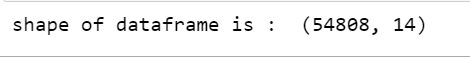
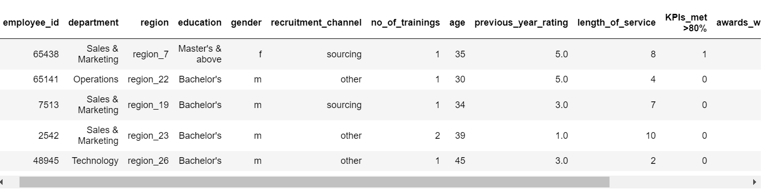
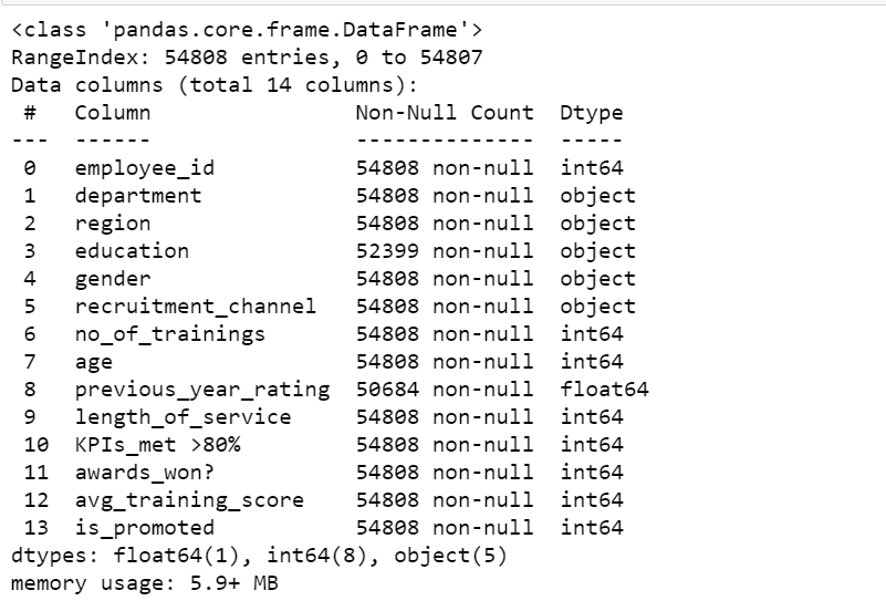
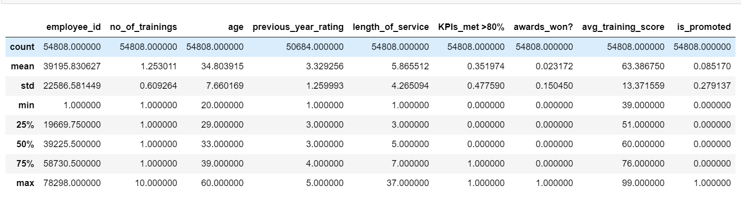
There are a total of 14 variables in this dataset, with a total of 54808 observations. “is_promoted” is our Target Variable, which has two categories encoded as 1 (promoted) and 0 (not promoted) rest all are input features. In addition, we can observe that our dataset contains both numerical and Categorical features.
Data Cleaning
Data cleaning is a crucial stage in the data preprocessing process. We’ll remove columns with only one unique value because their variance will be 0 and they won’t help us anticipate anything.
Let’s see whether there are any columns that
only have one unique value.
#Checking the unique value counts in columns
featureValues={}
for d in data.columns.tolist():
    count=data[d].nunique()
    if count==1:
        featureValues[d]=count
# List of columns having same 1 unique value
cols_to_drop= list(featureValues.keys())
print("Columns having 1 unique value are :n",cols_to_drop)
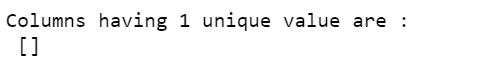
This signifies that there isn’t any column having only 1 unique value.
We’ll now drop the employee_id column because it’s merely a unique identifier, and
then verify each field in the dataset for null value percentages.
#Drop employee_id column as it is just a unique id
data.drop("employee_id",inplace=True,axis=1)
#Checking null percentage
data.isnull().mean()*100
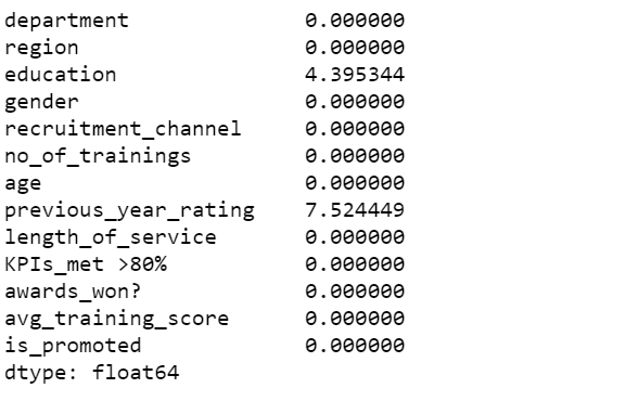
previous_year_rating and education both features have null values. As a result, we will impute those null values instead of dropping them. Following our examination of those columns, we discovered that –
- For rows with a null previous_year_rating, we can see that their length of service is 1, which could be why they don’t have a previous year rating. As a result, we’ll use 0 to impute null values.
- For the education column, we will impute null values with mode.
#fill missing value
data["previous_year_rating"]= data["previous_year_rating"].fillna(0)
#change type to int
data["previous_year_rating"]= data["previous_year_rating"].astype("int")
#Find out mode value for education
data["education"].mode()
#fill missing value with mode
data["education"]= data["education"].fillna("Bachelor's")
Now, we do not have any null or missing values in our data. So, let’s
proceed to our next step. There are no null or
missing values in our data now. So, let’s go on to the next step.
Exploratory Data Analysis before creating a Logistic Regression Model
Getting insights from data and visualizing them is an important stage in machine learning since it provides us with a better view of features and their relationships.
Let’s look at the target variable’s distribution in the dataset.
# cchart for distribution of target variable
fig= plt.figure(figsize=(10,3) )
fig.add_subplot(1,2,1)
a= data["is_promoted"].value_counts(normalize=True).plot.pie()
fig.add_subplot(1,2,2)
churnchart=sns.countplot(x=data["is_promoted"])
plt.tight_layout()
plt.show()
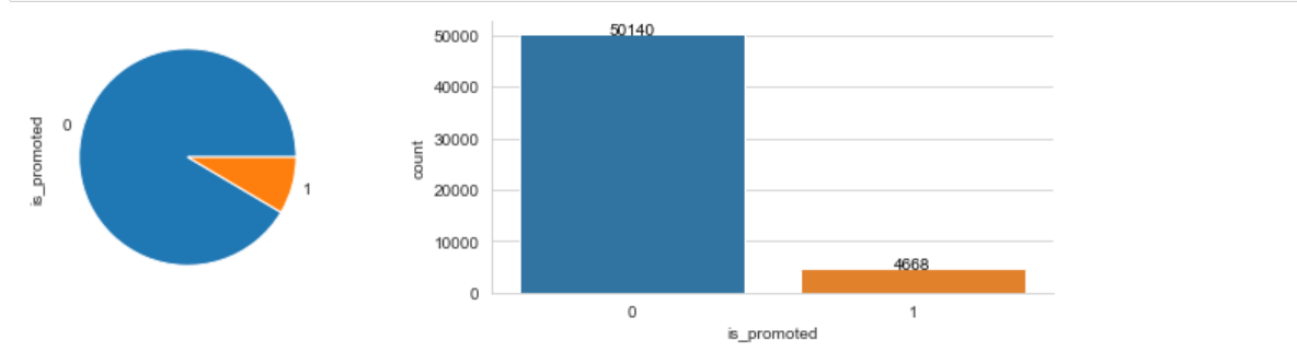
We can observe from the above charts that, promoted employee data is less than non-promoted employee data, indicating that there is a class imbalance because class 0 has more data points or observations than class.
Let’s visualize if there is any relationship between the target variable and other variables.
# Visualize relationship between promoted and other features
fig= plt.figure(figsize=(10,5) )
fig.add_subplot(1,3,1)
ar_6=sns.boxplot(x=data["is_promoted"],y=data["length_of_service"])
fig.add_subplot(1,3,2)
ar_6=sns.boxplot(x=data["is_promoted"],y=data["avg_training_score"])
fig.add_subplot(1,3,3)
ar_6=sns.boxplot(x=data["is_promoted"],y=data["previous_year_rating"])
plt.tight_layout()
plt.show()
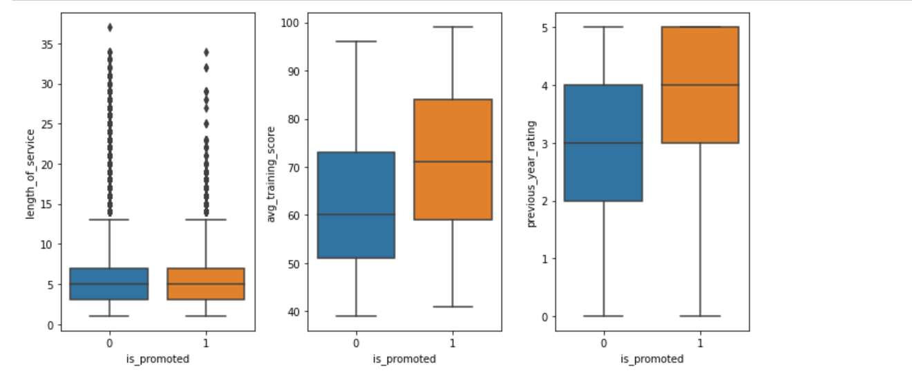
For an employee If the avg_training_score value is higher then the chances of getting promoted are more.
We will plot correlations between different variables using a heatmap.
#correlation between features
corr_plot = sns.heatmap(data.corr(),annot = True,linewidths=3 )
plt.title("Correlation plot")
plt.show()
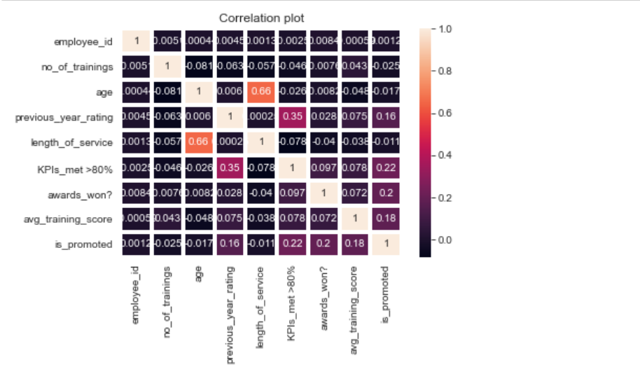
None of the features is highly correlated with each other except age and length of
the service.
Feature Engineering
In feature engineering, we apply domain expertise to produce new features from raw data, or we convert or encode features. We’ll encode categorical features or make dummy features out of them in this section.
#Converting Categorical columns into one hot encoding
data["gender"]=data["gender"].apply(lambda x: 1 if x=="m" else 0)
#list of columns
cols = data.select_dtypes(["object"]).columns
#Create dummy variables
ds=pd.get_dummies(data[cols],drop_first=True)
ds
#concat newly created columns with original dataframe
data=pd.concat([data,ds],axis=1)
#Drop original columns
data.drop(cols,axis=1,inplace=True)
Train-Test Split
We will divide the dataset into two subsets: train and test. To perform the train-test split, we’ll use Scikit-learn machine learning.
- Train subset – we will use this subset to fit/train the model
- Test subset – we will use this subset to evaluate our model
from sklearn.model_selection import train_test_split
#split data into dependent variables(X) and independent variable(y) that we would predict
y = data.pop("is_promoted")
X = data
#Let’s split X and y using Train test split
X_train,X_test,y_train,y_test = train_test_split(X,y,random_state=42,train_size=0.8)
#get shape of train and test data
print("train size X : ",X_train.shape)
print("train size y : ",y_train.shape)
print("test size X : ",X_test.shape)
print("test size y : ",y_test.shape)
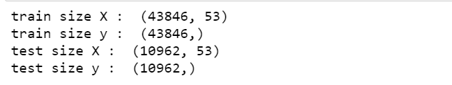
After splitting the dataset, we have 43846 observations in the training subset and 10962 in the test subset.
After diving into the dataset let’s move on to the next phase of feature scaling.
Feature Scaling/Normalization
Why Feature scaling is important?
As previously stated, Logistic Regression uses Gradient Descent as one of the approaches for obtaining the best result, and feature scaling helps to speed up the Gradient Descent convergence process. When we have features that vary greatly in magnitude, the algorithm assumes that features with a large magnitude are more relevant than those with a small magnitude. As a result, when we train the model, those characteristics become more important.
Because of this feature scaling is required to put all features into the same range, regardless of their relevance.
Feature Scaling Techniques
We bring all the features into the same range using feature scaling. There are many ways to do feature scaling like normalization, standardization, robust scaling, min-max scaling, etc. But here we will discuss the Standardization technique that we are going to apply to our features.
In standardization, features will be scaled to have a mean of 0 and a standard deviation of 1. It does not scale to a preset range. The features are scaled using the formula below:
z = (x – u) / s
where u is the mean of the training samples and s is a standard deviation of the training samples.
Let’s see how to do feature scaling in python using Scikit-learn.
#Feature scaling
from sklearn.preprocessing import StandardScaler
scale=StandardScaler()
X_train = scale.fit_transform(X_train)
X_test = scale.transform(X_test)
Class Imbalance
What is the class imbalance?
when a dataset has more data points or
observations belonging to one category and very few for another, we call
it a class imbalance problem since the distribution of class labels is
not balanced and skewed. Let’s see whether we have a class imbalance problem.
#check for distribution of labels
y_train.value_counts(normalize=True)
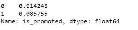
We can observe that the majority of the labels are from class 0 and only a few are from class 1.
If we use this distribution to develop our model, it may become biased towards predicting the majority class since there will be insufficient data to learn minority class patterns. The model will start predicting every new observation as 0 or majority class. (In our problem employee is not promoted). We’ll get more model accuracy here, but it won’t be a decent model because it won’t predict class 1 or minority class, which is a crucial class.
As a result, we must consider class imbalance when developing our Logistic Regression model.
How to Handle Class Imbalance?
There are a variety of approaches to dealing with class imbalance, such as increasing minority class samples or decreasing majority class samples to ensure that both classes have the same distribution.
Because we’re using the Scikit-learn machine library to create the model, it has a logistic regression implementation that supports class weighting. We will use the inbuilt parameter “class_weight” while creating an instance of the Logistic Regression model.
Both the majority and minority classes will be given separate weights. During the training phase, the weight differences will influence the classification of the classes.
The purpose of adding class weights is to penalize the minority class for misclassification by setting a higher class weight while decreasing the weight for the majority class.
Build and Train Logistic Regression model in Python
o implement Logistic Regression, we will use the Scikit-learn library. We’ll start by building a base model with default parameters, then look at how to improve it with Hyperparameter Tuning.
As previously stated, we will use the “class_weight” parameter to address the problem of class imbalance. Let’s start by creating our base model with the code below.
#import library
from sklearn.linear_model import LogisticRegression
#make instance of model with default parameters except class weight
#as we will add class weights due to class imbalance problem
lr_basemodel =LogisticRegression(class_weight={0:0.1,1:0.9})
# train model to learn relationships between input and output variables
lr_basemodel.fit(X_train,y_train)
After training our model on the training dataset, we used our model to predict values for the test dataset and recorded them in the y_pred_basemodel variable.
Let’s look at which metrics to use and how to evaluate our base model.
Model Evaluation Metrics
To evaluate performance or our model we will be using “f1 score” as this is a class imbalance problem using accuracy as a performance metrics is not good also, we can say that f1 score is the go-to metric when we have a class imbalance problem. The formula for calculating the F1 score is as follows:
F1 Score = 2*(Recall * Precision) / (Recall + Precision)
Precision is the ratio of accurately predicted positive observations to the total predicted positive observations.
Precision = TP/TP+FP
Recall is the ratio of accurately predicted positive observations to all observations in actual class – yes.
Recall = TP/TP+FN
F1 Score is the weighted average of Precision and Recall. Therefore, this score takes both false positives and false negatives into account.
Let’s evaluate our base model using the f1 score.
from sklearn.metrics import f1_score
print("f1 score for base model is : " , f1_score(y_test,y_pred_basemodel))

We got a 0.37 f1 score on our base model created using default parameters.
Up to this point, we saw how to create a logistic regression model using default parameters.
Now let’s increase model performance and evaluate it again after tuning hyperparameters of the model.
Hyperparameter Optimization for the Logistic Regression Model
Model parameters (such as weight, bias, and so on) are learned from data, whereas hyperparameters specify how our model should be organized. The process of finding the optimum fit or ideal model architecture is known as hyperparameter tuning. Hyperparameters control the overfitting or underfitting of the model. Hyperparameter tuning can be done using algorithms like Grid Search or Random Search.
We will use Grid Search which is the most basic method of searching optimal values for hyperparameters. To tune hyperparameters, follow the steps below:
- Create a model instance of the Logistic Regression class
- Specify hyperparameters with all possible values
- Define performance evaluation metrics
- Apply cross-validation
- Train the model using the training dataset
- Determine the best values for the hyperparameters given.
We can use the below code to implement hyperparameter tuning in python using the Grid Search method.
#Hyperparameter tuning
# define model/create instance
lr=LogisticRegression()
#tuning weight for minority class then weight for majority class will be 1-weight of minority class
#Setting the range for class weights
weights = np.linspace(0.0,0.99,500)
#specifying all hyperparameters with possible values
param= {'C': [0.1, 0.5, 1,10,15,20], 'penalty': ['l1', 'l2'],"class_weight":[{0:x ,1:1.0 -x} for x in weights]}
# create 5 folds
folds = StratifiedKFold(n_splits = 5, shuffle = True, random_state = 42)
#Gridsearch for hyperparam tuning
model= GridSearchCV(estimator= lr,param_grid=param,scoring="f1",cv=folds,return_train_score=True)
#train model to learn relationships between x and y
model.fit(X_train,y_train)
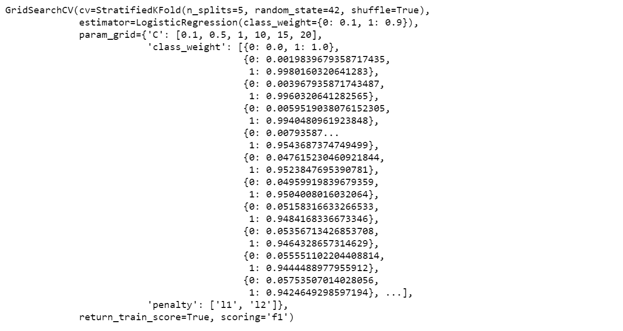
After fitting the model, we will extract the best fit values for all specified hyperparameters.
# print best hyperparameters
print("Best F1 score: ", model.best_score_)
print("Best hyperparameters: ", model.best_params_)

We will now build our Logistic Regression model using the above values we got by tuning Hyperparameters.
Build Model using optimal values of Hyperparameters
Let’s use the below code to build our model again.
#Building Model again with best params
lr2=LogisticRegression(class_weight={0:0.27,1:0.73},C=20,penalty="l2")
lr2.fit(X_train,y_train)

After training our final model it’s time to evaluate our Logistic Regression model using chosen metrics.
Model Evaluation
We will evaluate our model on Test Dataset. First, we will predict values on the Test dataset.
We chose “f1 score” as our performance metric above, but let’s look at the scores for all of the metrics, including confusion metrics, precision, recall, ROC-AUC score, and ultimately f1 score, for learning purposes.
Then, we’ll compare our final model’s f1 score to our base model to see if it’s improved.
We’ll use the code below to calculate the score
for various metrics:
# predict probabilities on Test and take probability for class 1([:1])
y_pred_prob_test = lr2.predict_proba(X_test)[:, 1]
#predict labels on test dataset
y_pred_test = lr2.predict(X_test)
# create onfusion matrix
cm = confusion_matrix(y_test, y_pred_test)
print("confusion Matrix is :nn",cm)
print("n")
# ROC- AUC score
print("ROC-AUC score  test dataset:  t", roc_auc_score(y_test,y_pred_prob_test))
#Precision score
print("precision score  test dataset:  t", precision_score(y_test,y_pred_test))
#Recall Score
print("Recall score  test dataset:  t", recall_score(y_test,y_pred_test))
#f1 score
print("f1 score  test dataset :  t", f1_score(y_test,y_pred_test))
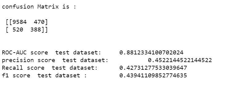
We can see that by tuning hyperparameters, we were able to improve the performance of our model since our F1 Score for the final model (0.43) is higher than that of the base model (0.37). After the hyperparameter tuning model got a 0.88 ROC-AUC score.
With this, we were able to construct our logistic regression model and test it on the Test dataset. More feature engineering, hyperparameter optimization, and cross-validation techniques can improve its performance even more.
Conclusion
We began our learning journey by understanding the basics of machine learning and logistic regression. Then we moved on to the implementation of a Logistic Regression model in Python. We learned key steps in Building a Logistic Regression model like Data cleaning, EDA, Feature engineering, feature scaling, handling class imbalance problems, training, prediction, and evaluation of model on the test dataset. Apart from that, we learned how to use Hyperparameter Tuning to improve the performance of our model and avoid overfitting and underfitting.
I hope you find this information useful and will try it out.
Connect with me on LinkedIn.
The media shown in this article are not owned by Analytics Vidhya and are used at the Author’s discretion.
Size: Unknown Price: Free Author: yogitaBhor Data source: https://www.analyticsvidhya.com/