Complete guide on how to Use LightGBM in Python
- by user1
- 21 March, 2022
This article was published as a part of the Data Science Blogathon
Introduction
A Gradient Boosting Decision tree or a GBDT is a very popular machine learning algorithm that has effective implementations like XGBoost and many optimization techniques are actually adopted from this algorithm. The efficiency and scalability of the model are not quite up to the mark when there are more features in the data. For this specific behavior, the major reason is that each feature should scan all the various data instances to make an estimate of all the possible split points which is very time-consuming and tedious.
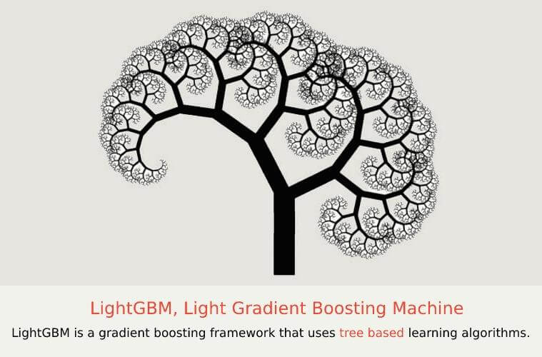
Source: https://s3.ap-south-1.amazonaws.com/techleerimages/0504748b-5e9b-49ee-9824-3ab4ac76760e.jpg
To solve this problem, The LGBM or Light Gradient Boosting Model is used. It uses two types of techniques which are gradient Based on side sampling or GOSS and Exclusive Feature bundling or EFB. So GOSS will actually exclude the significant portion of the data part which have small gradients and only use the remaining data to estimate the overall information gain. The data instances which have large gradients actually play a greater role for computation on information gain. GOSS can get accurate results with a significant information gain despite using a smaller dataset than other models.
With the EFB, It puts the mutually exclusive features along with nothing but it will rarely take any non-zero value at the same time to reduce the number of features. This impacts the overall result for an effective feature elimination without compromising the accuracy of the split point.
By combining the two changes, it will fasten up the training time of any algorithm by 20 times. So LGBM can be thought of as gradient boosting trees with the combination for EFB and GOSS. You can access their official documentation here.
The main features of the LGBM model are as follows :
- Higher accuracy and a faster training speed.
- Low memory utilization
- Comparatively better accuracy than other boosting algorithms and handles overfitting much better while working with smaller datasets.
- Parallel Learning support.
- Compatible with both small and large datasets
With the above-mentioned features and advantages of LGBM, it has become the default algorithm for machine learning competitions when someone is working with a tabular kind of data regarding both regression and classification problems.
Demystifying the Maths behind LGBM
We use a concept known as verdict trees so that we can cram a function like for example, from the input space X, towards the gradient space G. A training set with the instances like x1,x2 and up to xn is assumed where each element is a vector with s dimensions in the space X. In each of the restatements of a gradient boosting, all the negative gradients of a loss function with respect towards the output model are denoted as g1, g2, and up to gn. The decision tree actually divides each and every node at the most revealing feature, it also gives rise to the largest evidence gain. In this type of model, the data improvement can be measured by the variance after segregating. It can be represented by the following formula :
“Y=Base_tree(X)-lr*Tree1(X)-lr*Tree2(X)-lr*Tree3(X)”
Explanation, Let O be a training dataset on a fixed node of a decision tree and then the variance gain of dividing measure j at a point d for a node is defined as :
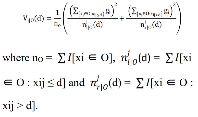
Source: https://ejmcm.com/article_9403_15c24bd9c676c28d90c3fc5fad8b42ea.pdf
Gradient One-Sided Sampling or GOSS utilizes every instance with a larger gradient and does the task of random sampling on the various instances with the small gradients. The training dataset is given by the notation of O for each particular node of the Decision tree. The variance gain of j or the dividing measure at the point d for the node is given by :
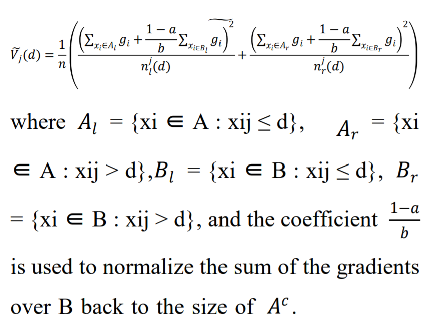
Source: https://ejmcm.com/article_9403_15c24bd9c676c28d90c3fc5fad8b42ea.pdf
This is achieved by the method of GOSS in LightGBM models.
Coding an LGBM in Python
The LGBM model can be installed by using the Python pip function and the command is “pip install lightbgm” LGBM also has a custom API support in it and using it we can implement both Classifier and regression algorithms where both the models operate in a similar fashion. The Dataset used here is of the Titanic Passengers which will be used in the below code and can be found in my drive at this location.
( Dataset Link: https://drive.google.com/file/d/1uuFe0f2gjEE77-PL9LhMrEd6n-1L5vfW/view?usp=sharing )
Code :
Importing all the libraries
import lightgbm as lgb
import pandas as pd
import numpy as np
from sklearn.model_selection import train_test_split
from sklearn import metrics
Loading the Data :
data = pd.read_csv('/content/SVMtrain.csv')
data.head()
Output :
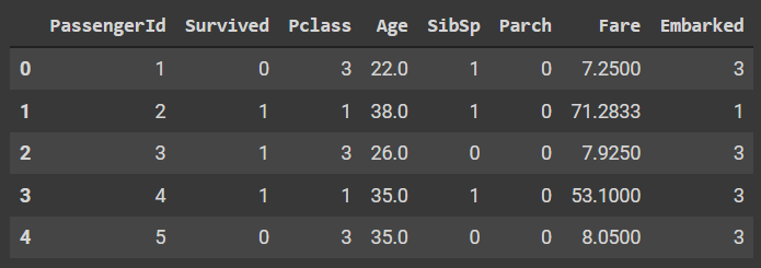
Here we can see that there are 8 columns out of which the passenger ID will be dropped and the embarked will be finally chosen as a target variable for the following classification challenge.
Loading the variables:
# To define the input and output feature
x = data.drop(['Embarked','PassengerId'],axis=1)
y = data.Embarked
# train and test split
x_train,x_test,y_train,y_test = train_test_split(x,y,test_size=0.33,random_state=42)
Loading and fitting the model:
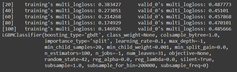
The initial process of initializing a model is very similar to a normal model initializing and the main difference is that we will get much more parameter settings adjustments while we are initializing the model. We will define the max_depth, learning rate and random state in the following code. In the fit model, we have passed eval_matrix and eval_set to evaluate the model during training itself.
Code :
model = lgb.LGBMClassifier(learning_rate=0.09,max_depth=-5,random_state=42)
model.fit(x_train,y_train,eval_set=[(x_test,y_test),(x_train,y_train)],
          verbose=20,eval_metric='logloss')
Output:
Since our model has very low instances, we need to first check for overfitting with the following code and then we will proceed for the next few steps :
Code :
print('Training accuracy {:.4f}'.format(model.score(x_train,y_train)))
print('Testing accuracy {:.4f}'.format(model.score(x_test,y_test)))
Output :
Training accuracy 0.9647
Testing accuracy 0.8163
As we can clearly see that there is absolutely no significant difference between both the accuracies and hence the model has made an estimation that is quite accurate.
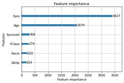
LGBM also comes with additional plotting functions like plotting the various feature importance, metric evaluation and the tree plot.
Code :
lgb.plot_importance(model)
Output :
If you do not mention the eval_set during the fitment, then you will actually get an error while plotting the metric evaluation
Code :
lgb.plot_metric(model)
Output
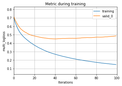
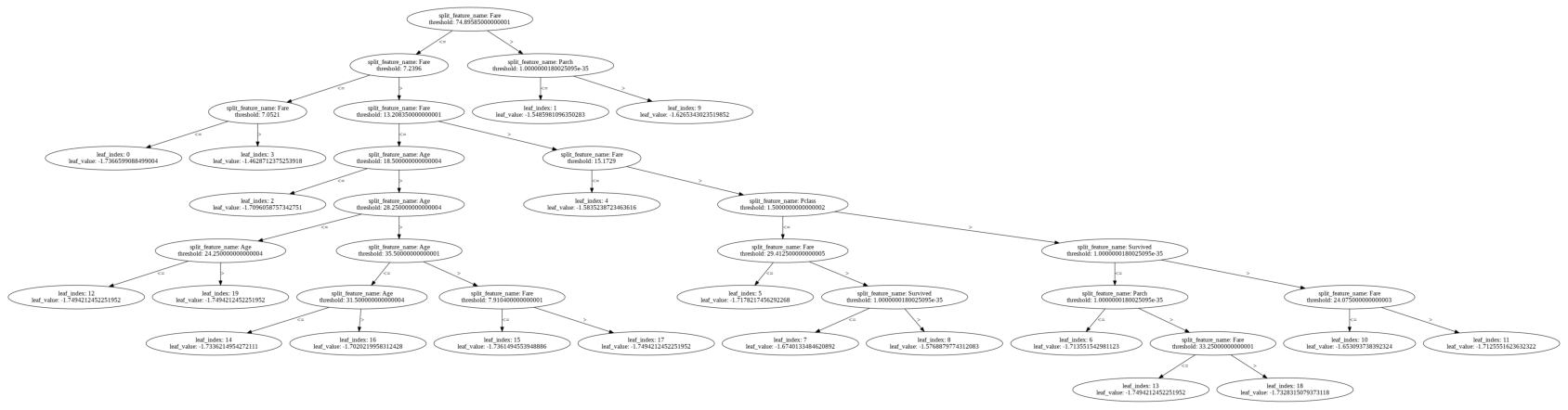
And as you can clearly see here, the validation curve will tend to increase after it has crossed the 100th evaluation. This can be totally fixed by tuning and setting the hyperparameters of the model. We can also plot the tree using a function.
Code:
lgb.plot_tree(model,figsize=(30,40))
Output:
Now we will plot a few metrics by using the sklearn library
Code :
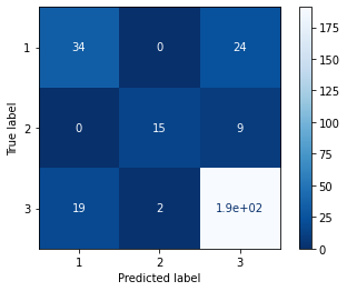
metrics.plot_confusion_matrix(model,x_test,y_test,cmap='Blues_r')
Output :
Code :
print(metrics.classification_report(y_test,model.predict(x_test)))
Output :
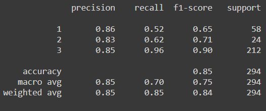
Now as we can clearly see from the confusion matrix combined with the classification report, the model is struggling to predict class 1 because of the few instances that we have but if we compare the same result with the other various ensemble algorithm, then LGBM performs the best. We can also perform the same process for the regressor model but there we need to change the estimator to the LGBMRegressor()
End Notes:
From this article, we can see and understand how to use an LGBM model and how it can tackle the problem by using a GODD and EFB and then we implemented it for a real-life classification problem and the overall process is also very similar to the other ML algorithms. The in-built plotting functionality also makes the library much more attractive and reduces the overall effort for the evaluation side.
Stay Safe and get vaccinated everyone.
Arnab Mondal
Data Engineer | Python Developer
https://www.linkedin.com/in/arnab1408/
Collab Notebook Link :
https://colab.research.google.com/drive/1KJAGA3NRyy7wMPEWPnBo1ooMOJtvKcrG?usp=sharingThe media shown in this article are not owned by Analytics Vidhya and are used at the Author’s discretion.
Size: Unknown Price: Free Author: Arnab Mondal Data source: https://www.analyticsvidhya.com/