A Beginners Guide To Statistics for Machine Learning!

by user1
21 March, 2022

This article was published as a part of the Data Science Blogathon

As Karl Pearson, a British mathematician has once stated, Statistics is the grammar of science, especially for computers and IT, physics, and biology. When one starts a journey in Data Science or Data Analytics, having statistical knowledge will have the leverage to get better data insights from the data.

“Statistics is that the grammar of science.” Karl Pearson

The importance of statistics in Data Science and Data Analytics can’t be underestimated. Statistics provides tools and methods to seek out structure and to offer deeper data insights. Knowing Statistics well will allow you to think critically, and be creative when using the info to unravel business problems and make data-driven decisions. In this article, we will try to cover the following Statistics topics for data science and data analytics:

Random Variables:

A random variable is simply a way to map the outcomes of random processes, such as flipping a coin or rolling dice, or selecting a card from a pack of cards, to numbers. For example, consider the random process of flipping a coin by random variable X which takes a value of 1 if the outcome if heads and 0 if the outcome is tails.

There are two types of random variables Discrete Random Variable and Continuous Random Variable.

Discrete Random Variable is the one that takes which may take a countable number of distinct values(not necessarily that we can count). E.g 1,2,3,…., Number of days in a week, Number of students in a school. The Continuous Random Variable can take infinitely many values. E.g Heights, weights, temperature, distance, etc.

Probability:

The set of possible outcomes is called the sample space of the random variable. Each time the random process is repeated is called an Event. The chance or the likelihood of an event occurring with a particular outcome is called the probability of that event. A probability of an event is the chance or likelihood that a random variable takes a specific value of x which can be described by P(x).

We will take the above-mentioned example of flipping a coin again, the likelihood of getting heads or tails is the same, that is 0.5 or 50%. So we have the following setting:

Population and Sample:

The population is an entire collection of all items/entities that you want to conclude insights about. It is usually very large and diverse. Generally, it is denoted by ‘N’.A sample is the subset of the population that represents it and is denoted by ‘n’. The size of the sample will be always less than the size of the population.The population doesn’t always necessarily refers to people. It may be a group containing elements such as objects, countries, species, etc.

Measures of Central Tendency:

Mean:

The mean is the arithmetic average of all data points or observations in the given data set.

Calculating the mean is very simple, you just add up all the values and divide by the total number of values in the dataset.

where N is the number of data points or observations in the sample. The sample mean is denoted by μ, which is very often used to approximate the population mean, which is expressed above.

Median:

Simply, the median is the middle value in the dataset. The value that splits the data in half.

Mode:

The mode is the most frequent value that occurs in the dataset.

Image Source

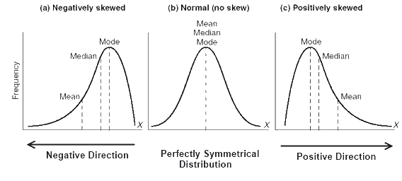
If the distribution of data is skewed to the left(Negatively skewed), the mean is less than the median, which is often less than the mode.
(median < median < mode)
If the distribution of data is skewed to the right(Positively skewed), the mode is often less than the median, which is less than the mean.
(mean > median > mode)
If the distribution of data is symmetric, mode = median = mean.

Variance:

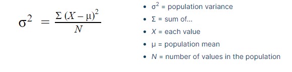
Simply, you can refer to the variance as a statistical measure of the spread of variables in the dataset.

More specifically, it measures how far a variable in the dataset is from the mean. It is denoted by

(for population mean).

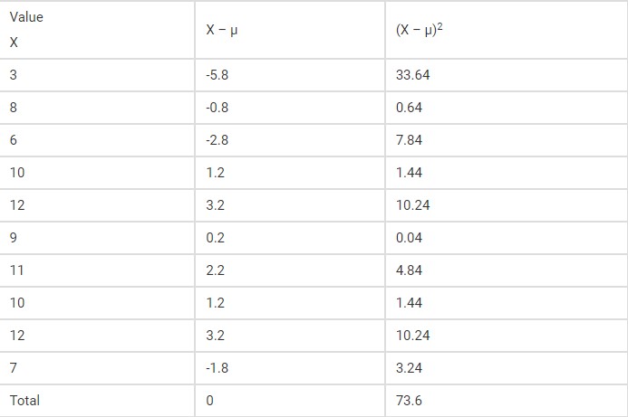
Example: Find the variance of the numbers 3, 8, 6, 10, 12, 9, 11, 10, 12, 7.

Solution:

Given,

3, 8, 6, 10, 12, 9, 11, 10, 12, 7

Step 1: Compute the mean of the 10 values given.

Mean = (3+8+6+10+12+9+11+10+12+7) / 10

= 88 / 10

= 8.8

Step 2: Make a table with three columns, one for the X values, the second for the deviations, and the third for squared deviations. As the data is not given as sample data so we use the formula for population variance. Thus, the mean is denoted by μ.

Step 3: Calculate Variance by substituting the values in the formula,

Standard deviation:

Standard deviation is a quantity that expresses how much a variable of dataset differs from the mean. It is denoted by

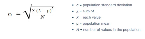
Standard deviation is often preferred over the variance because it has the same unit as the data points, which means you can interpret it more easily.

Example:

A hen lays eight eggs. Each egg was weighed and recorded as follows:

60 g, 56 g, 61 g, 68 g, 51 g, 53 g, 69 g, 54 g. Find the Standard deviation.

First, calculate the mean:

2.Now, find the standard deviation

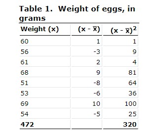
Using the information from the above table, we can see that

To calculate the standard deviation, we must use the following formula:

Therefore, standard deviation = 6.32g

Correlation, Causation, and Covariance:

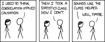
The correlation is the term in statistics that refers to the relationship (i.e. degree of association between two random variables) and it measures both the strength as well as the direction of the linear relationship between two variables. Correlation tells us how well a pair of numeric variables are linearly related, but it doesn’t give us the reason behind that relationship. If a correlation is present between two variables then it means that there is a relationship or a pattern between the values of the two target variables. But this doesn’t imply that the two variables cause each other (i.e. Change in one variable will cause the change in another variable. )

Correlation coefficients’ values range between -1 and 1. Note that the correlation of a variable with itself is always 1, that is Cor(X, X) = 1. Note that when interpreting correlation do not confuse it with causation, given that a correlation is not causation. Even if there is a correlation between two variables, you can’t conclude that one variable causes a change in the other.

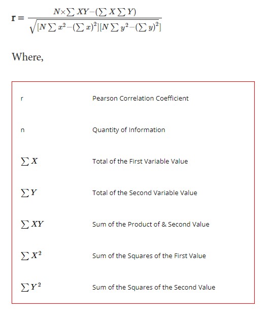
The most common formula used for linear dependency between the data set is Pearson’s Correlation coefficient.

Formula :

Image Soure

Example: Calculate the correlation coefficient for the following data:

X = 4, 8 ,12, 16 and

Y = 5, 10, 15, 20.

Solution:

Given variables are,

X = 4, 8 ,12, 16 and

Y = 5, 10, 15, 20

To find the linear coefficient of these data, we need to first construct a table as follows to get the required values of the formula.

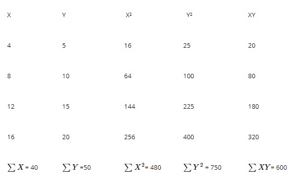
Putting all the values in the formula,

Therefore, the correlation coefficient is 1.

Causation means that the two variables have a cause-and-effect relationship with one another. (E.g. Event A causes event B) It may also happen that the relationship could be coincidental, or a third factor might be causing both variables to change.

Image Source

The covariance is a statistical measure of the relationship between two random variables. It evaluates how much – to what extent – the variables change together.

Covariance can take negative or positive values as well as zero. A positive value of covariance indicates that two random variables tend to vary within the same direction, whereas a negative value suggests that these variables vary in opposite directions. Finally, the value zero means that they don’t vary together.

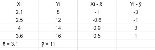
Example: The table below describes the rate of economic growth (xi) and the rate of return on the S&P 500 (y_i). Using the covariance formula, determine whether economic growth and S&P 500 returns have a positive or inverse relationship. Before you compute the covariance.

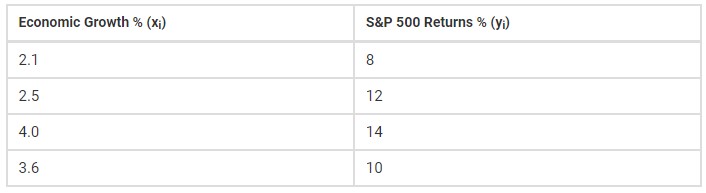
x = 2.1, 2.5, 4.0, and 3.6 (economic growth)

y = 8, 12, 14, and 10 (S&P 500 returns)

Solution:

We need to first construct a table as follows to get the required values of the formula.

Covariance and correlation both primarily assess the relationship between two variables. But they are not the same.

Covariance measures the variation of two random variables from their expected values. However, it doesn’t indicate the strength of the relationship, nor the dependency between variables.

While, correlation measures how strong the relationship is, nor the dependency between variables. Simply, correlation is a scaled measure of covariance.

Relationship between correlation and covariance:

here

is a variance.

Discrete Probability Distributions:

A discrete distribution is a probability distribution that gives the discrete (individually countable) outcomes, such as 1, 2, 3… There are many discrete probability distributions to be used in different scenarios. We will discuss some of the Discrete distributions below:

Binomial Distribution:

The binomial distribution gives the discrete probability distribution P(X = r) of obtaining exactly rsuccesses out of n Bernoulli trials (where the result of each Bernoulli trial is true with probability pand false with probability 1 − p ). The binomial distribution is given by,

where nCr means the number of ways of choosing r unordered outcomes from n possibilities. You can find more about combination here.

To be able to apply the binomial formula the following conditions needs to be satisfied,

The total number of trials should be fixed at n.
The n trials are independent.
Each trial is binary, that is it has only two possible outcomes, success or failure.
The probability of success is the same in all trials, denoted by p.
The random variable X is the number of successes in the n trials.

Example: A coin is tossed 10 times. What is the probability of getting exactly 6 heads?

Solution: Here we will be using Binomial distribution.

Because the number of trials is fixed, and independent. Each trial is binary (heads or tails). The probability of success for each trial is the same (i.e. P(Heads) = 0.5 ). So all the above conditions are satisfied.

The number of trials (n) = 10
The odds of success (“tossing a heads”) = 0.5

(1 – p) = 1 – 0.5 = 0.5

X = 6 ( where the random variable X represents the probability of getting exactly 6 heads)

Substituting all the values in above formula

P(X = 6) = ¹⁰C₆ * 0.5⁶ * 0.5⁴

= 210 * 0.015625 * 0.0625

= 0.205078125

Negative Binomial Distribution:

Similarly, if X denotes the number of trials until the r^th success, then the probability distribution is given by,

Example: Robert is a football player. His success rate of goal hitting is 70%. What is the probability that Robert hits his third goal on his fifth attempt?

Solution:

Here probability of success, P is 0.70. The number of trials n is 5, and the number of successes, r is 3. Using the negative binomial distribution formula, let’s compute the probability of hitting the third goal in the fifth attempt.

Substituting all the values in above formula, we get

P( X = 3 ) = ^5-1C_3-1 * (0.7)³ * (0.3)^5-3

= ⁴C₂ * (0.7)³ * (0.3)²

= 6 * 0.343 * 0.09

= 0.185

Therefore, the probability that Robert hits his third goal on his fifth attempt is 0.185.

Geometric Distribution:

A geometric distribution is a special case of a negative binomial distribution with r = 1 . Let Xdenote the number of trials until the first success, then the probability distribution is given by,

Example: In an amusement fair, a competitor is entitled for a prize if he throws a ring on a peg from a certain distance. It is observed that only 30% of the competitors can do this. If someone is given 5 chances, what is the probability of his winning the prize when he has already missed 4 chances?

Solution:

If someone has already missed four chances and has to win in the fifth chance, then it is a probability experiment of getting the first success in 5 trials. The problem statement also suggests the probability distribution be geometric.

Here,

p = 30% = 0.3

( 1 – p ) = 1 – 0.3 = 0.7

n = 5

Substituting all the values in the above formula, we get

Therefore, the probability of his winning the prize when he has already missed 4 chances is 0.072 i.e. 7.2%

Poisson Distribution:

Let the discrete random variable X denote the number of times an event occurs in an interval oftime (or space). Then X may be a Poisson random variable with r = 0, 1, 2…, λ > 0 ( λ being boththe mean and the variance of X ) and the probability distribution is given by,

Example: As only 3 students came to attend the class today, find the probability for exactly 4 students to attend the classes tomorrow.

Solution:

Given,
Average rate of value(λ) = 3
Poisson random variable(r) = 4

Poisson distribution = P(X = r) =

P( X = 4 ) =

P(X=4) = 0.16803135574154

Bernoulli Distribution:

Bernoulli distribution has two possible outcomes- success and failure. The simplest example for Bernoulli Distribution is flipping a coin. It has two possible outcomes only-heads or tails.

Let p be the probability of success and 1 – p is the probability of failure. Then PMF(Probability Mass Function) is given by,

Continuous Probability Distributions:

It is a probability distribution in which the random variable X can take on any value (is continuous). Because there are infinite values that X could assume, so the probability of X taking a specific value is zero.

Probability Density Functions:

For continuous random variables, as we discussed, the probability that X takes on any particular value x is 0. That is, finding for a continuous random variable X is not going to work. Instead, we need to find the probability of random variable X falls in some interval (a,b), that is, we’ll need to find P(a < X < b). We can achieve this by the Probability Density function.

Normal Distribution:

A normal ( Gaussian/ Gauss /Laplace-Gauss/ z ) distribution is a type of continuousprobability distribution for a real-valued random variable. A normal distribution is sometimesinformally called a bell curve.

In a normal distribution, the mean is zero and the standard deviation is one. It has zero skew and a kurtosis of 3. Normal distributions are symmetrical, but not all symmetrical distributions are normally distributed.

Normal distribution fits most of the natural phenomena.

You can read more about this here.

The Probability Density Function for normal distribution is given by,

where the parameter μ is the mean or expectation of the distribution and σ is its standard deviation. The variance of the distribution is σ².

Image Source

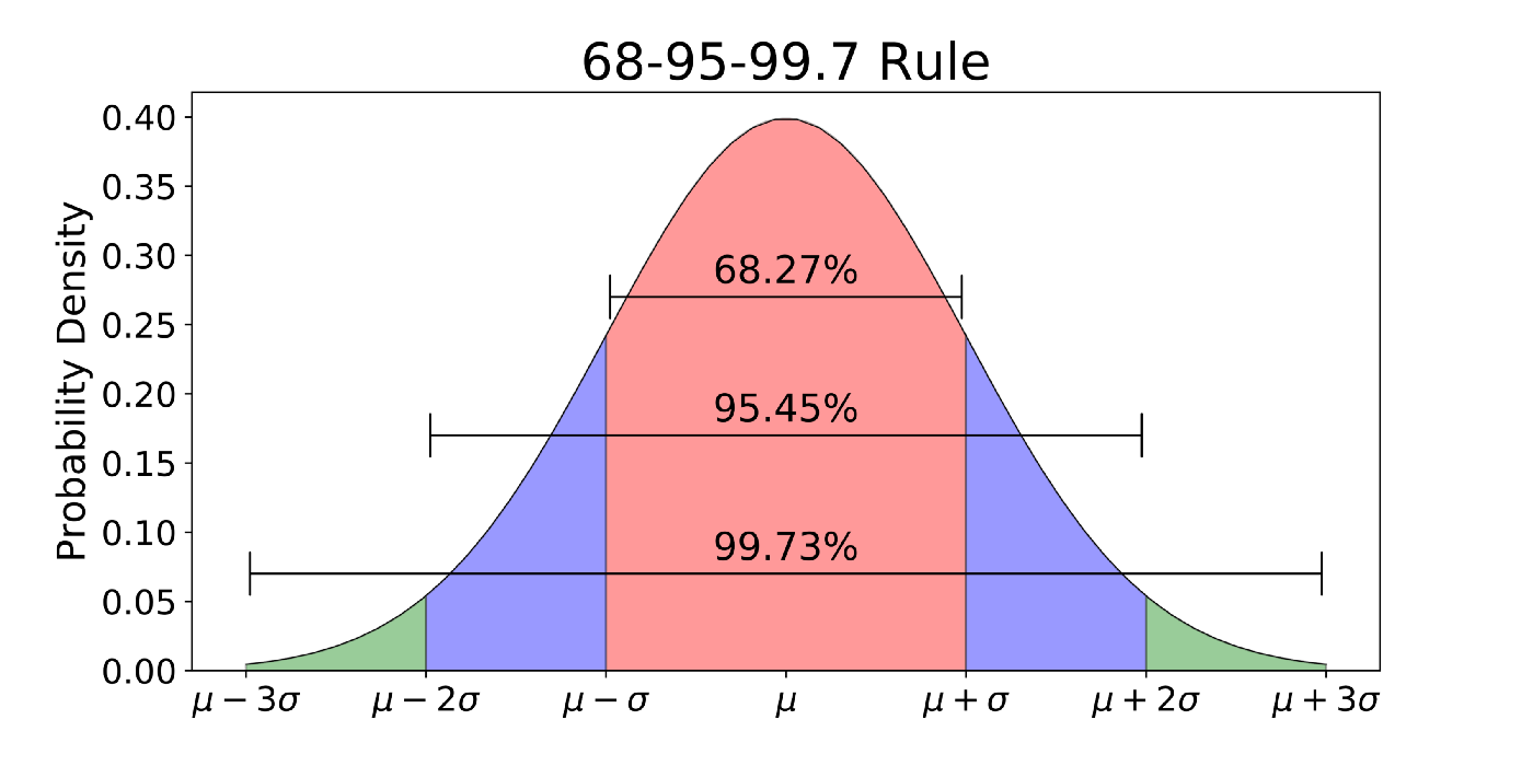
Any data that is normally distributed follow the 1-2-3 rule. This rule states that,

There is a 68.27 % probability of the variable lying within 1 standard deviation of the mean.
There is a 95.45 % probability of the variable lying within 2 standard deviations of the mean.
There is a 99.73 % probability of the variable lying within 3 standard deviations of the mean.

You can read more about examples here.

Standard Normal Distribution:

The standard normal distribution is a normal distribution with a mean of zero and a standard deviation of 1.And the probability density function is given by,

You can read more about this here.

Student’s T-Distribution:

The Student’sT distribution (also called T Distribution) is a family of distributions that look almost identical to the normal distribution curve, only a bit shorter and fatter. The t distribution is used when you have small samples. The more the sample size increases, the more the t distribution looks similar to the normal distribution. In fact, for sample sizes larger than 20, the distribution almost looks like the normal distribution.

Image Source

You can read more about this here.

Gamma Distribution:

The gamma distribution is another widely used distribution. It is important is due to its relationship with exponential and normal distributions. The continuous random variable X follows a gammadistribution for x (the waiting time) until the k^th event occurs if its probability density function is,

Image Source

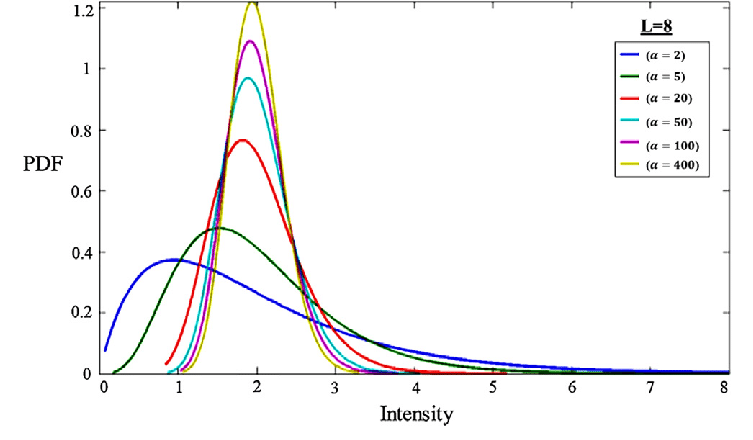
You can read more about this here.

Exponential Distribution:

It is one of the widely used continuous distributions. It is often used to model the time elapsed between events. The continuous random variable X follows an exponential distribution if its probability density function is,

The following figures give the PDF

Image Source

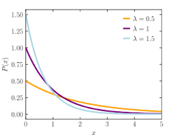
You can read more about this here.

Chi-Squared Distribution:

The chi-square distribution (also chi-squared or χ² -distribution) with k degrees of freedom is the distribution of a sum of the squares of k independent standard normal random variables. It is mostly used in hypothesis testing, inferential statistics, and to find confidence intervals. The continuous random variable X follows anchi-squared distribution if its PDF is,

The following figure gives the PDF,

Image Source

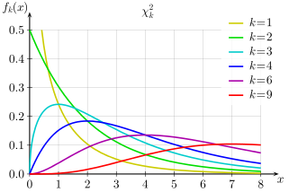
You can read more about this here.

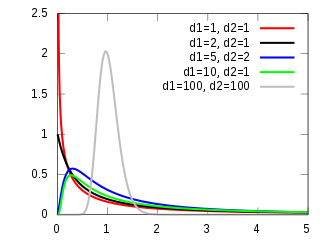
F-Distribution:

The F distribution is the probability distribution related to the f statistic. The distribution of all possible values of the f statistic is called an F distribution.

If a random variable X has an F-distribution with parameters d₁ and d₂. Then the PDF for X is given by

You can read more about this here.

The following figure gives the PDF,

Image Source

End!!!!!

Hope you enjoyed the article. Keep reading!!!…

If you liked this article, here are some other articles you may enjoy:

The media shown in this article are not owned by Analytics Vidhya and are used at the Author’s discretion.

Size: Unknown Price: Free Author: KAVITA MALI Data source: https://www.analyticsvidhya.com/