


This article was published as a part of the Data Science Blogathon
What is Anomaly Detection?
Anomaly detection detects anomalies in the data. Anomalies are the observations that deviate significantly from normal observations. Anomaly detection can be used in many areas such as Fraud Detection, Spam Filtering, Anomalies in Stock Market Prices, etc. Finding anomalies would help you in many ways. If you remove potential anomalies in the training data, the model is more likely to perform well. The very well-known basic way of finding anomalies is IQR (Inter-Quartile Range) which uses information like quartiles and inter-quartile range to find the potential anomalies in the data. Other algorithms include Isolation Forest, COPOD, KNN based anomaly detection, Auto Encoders, LOF, etc. These algorithms are predominantly used in non-time series anomaly detection.
Why do we need separate Anomaly Detection Algorithms for Time Series Data?
To answer the question above, we need to understand the concepts of time-series data. Time-series data are strictly sequential and have autocorrelation, which means the observations in the data are dependant on their previous observations. If we use standard algorithms to find the anomalies in the time-series data we might get spurious predictions. So the time-series data must be treated specially.
Steps followed to detect anomalies in the time series data are,
- Conduct an ADF test to check whether the data is stationary or not. If the data is not stationary convert the data into stationary data.
- After converting the data into stationary data, fit a time-series model to model the relationship between the data.
- Find the squared residual errors for each observation and find a threshold for those squared errors.
- Any observation’s squared error exceeding the threshold can be marked as an anomaly.
The reason behind using this approach,
As stated earlier, the time-series data are strictly sequential and contain autocorrelation. By using the above approach the model would find the general behaviour of the data. The normal data’s prediction error would be much smaller when compared to anomalous data’s prediction error.
Univariate Time Series Anomaly Detection vs. Multivariate Time Series Anomaly Detection
- Univariate time-series data consist of only one column and a timestamp associated with it. We use algorithms like AR (Auto Regression), MA (Moving Average), ARMA (Auto-Regressive Moving Average), and ARIMA (Auto-Regressive Integrated Moving Average) to model the relationship with the data.
- Multivariate time-series data consist of more than one column and a timestamp associated with it. We use algorithms like VAR (Vector Auto-Regression), VMA (Vector Moving Average), VARMA (Vector Auto-Regression Moving Average), VARIMA (Vector Auto-Regressive Integrated Moving Average), and VECM (Vector Error Correction Model).
Multivariate Time Series Anomaly Detection
We are going to use occupancy data from Kaggle. You can find the data here. The data contains the following columns date, Temperature, Humidity, Light, CO2, HumidityRatio, and Occupancy.
def test_stationarity(ts_data, column='', signif=0.05, series=False):
    if series:
        adf_test = adfuller(ts_data, autolag='AIC')
    else:
        adf_test = adfuller(ts_data[column], autolag='AIC')
    p_value = adf_test[1]
    if p_value <= signif:
        test_result = "Stationary"
    else:
        test_result = "Non-Stationary"
    return test_result
"""Multivariate Time Series"""
occ_data = pd.read_csv('datatest.txt')
occ_data = occ_data.set_index('date')
occ_data.head()

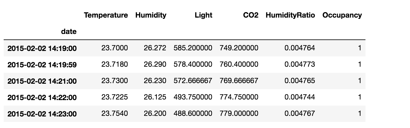
Image Source: Author’s Jupyter Notebook
First of all, we’re going to check whether each column of the data is stationary or not using the ADF (Augmented-Dickey Fuller) test. The ADF test provides us with a p-value which we can use to find whether the data is Stationary or not. If the p-value is less than the significance level then the data is stationary, or else the data is non-stationary.
adf_test_results = {
    col: test_stationarity(occ_data, col)
    for col in occ_data.columns
}
adf_test_results
# Output
# {'Temperature': 'Non-Stationary',
#  'Humidity': 'Non-Stationary',
#  'Light': 'Non-Stationary',
#  'CO2': 'Non-Stationary',
#  'HumidityRatio': 'Non-Stationary',
#  'Occupancy': 'Non-Stationary'}
We have run the ADF test for every column in the data. The test results show that all the columns in the data are non-stationary. So we need to convert the non-stationary data into stationary data.
There are multiple ways to convert the non-stationary data into stationary data like differencing, log transformation, and seasonal decomposition. In this post, we are going to use differencing to convert the data into stationary data.
def differencing(data, column, order):
    differenced_data = data[column].diff(order)
    differenced_data.fillna(differenced_data.mean(), inplace=True)
    return differenced_data
for col in occ_data.columns:
    occ_data[col] = differencing(occ_data, col, 1)
The code above takes every column and performs differencing operations of order one. Now, we have differenced the data with order one. Let’s check whether the data has become stationary or not.
adf_test_results = {
    col: test_stationarity(occ_data, col)
    for col in occ_data.columns
}
adf_test_results
# Output
# {'Temperature': 'Stationary',
#  'Humidity': 'Stationary',
#  'Light': 'Stationary',
#  'CO2': 'Stationary',
#  'HumidityRatio': 'Stationary',
#  'Occupancy': 'Stationary'}
Now all the columns in the data have become stationary. If the differencing operation didn’t convert the data into stationary try out using log transformation and seasonal decomposition to convert the data into stationary. Now we can fit a time-series model to model the relationship between the data. Here we’re going to use VAR (Vector Auto-Regression) model.
from statsmodels.tsa.api import VAR
max_lag = 20
var_model = VAR(occ_data)
# select the best lag order
lag_results = var_model.select_order(max_lag)
selected_lag = lag_results.aic
print(selected_lag) # selected_lag = 13
The select_order method of VAR is used to find the best lag for the data. In our case, the best order for the lag is 13, which gives us the minimum AIC value for the model.
The VAR model uses the lags of every column of the data as features and the columns in the provided data as targets. The VAR model is going to fit the generated features and fit the least-squares or linear regression by using every column of the data as targets separately. As stated earlier, the reason behind using this kind of method is the presence of autocorrelation in the data. If we use linear regression to directly model this it would end up in autocorrelation of the residuals, which would end up in spurious predictions.
def find_anomalies(squared_errors):
    threshold = np.mean(squared_errors) + np.std(squared_errors)
    predictions = (squared_errors >= threshold).astype(int)
    return predictions, threshold
var = VAR(occ_data)
var_fitresults = var.fit(selected_lag)
squared_errors = var_fitresults.resid.sum(axis=1) ** 2
predictions, threshold = find_anomalies(squared_errors) # threshold = 7593.829254818655
Now by using the selected lag, fit the VAR model and find the squared errors of the data. The squared errors are then used to find the threshold, above which the observations are considered to be anomalies.
The method used to find threshold is,
threshold = mean(squared_errors) + z * standard_deviation(squared_errors)
We can also use another method to find thresholds like finding the 90th percentile of the squared errors as the threshold. Here we have used z = 1, feel free to use different values of z and explore. The best value for z is considered to be between 1 and 10.
data = occ_data.iloc[selected_lag:, :]
data['Predictions'] = predictions.values
data

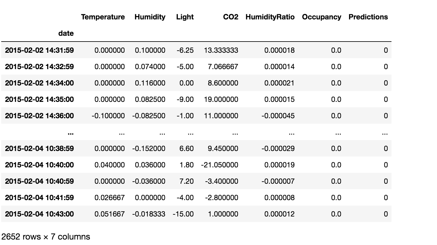
Image Source: Author’s Jupyter Notebook
data['Predictions'].value_counts()
# 0    2635
# 1      17
# Name: Predictions, dtype: int64
The model has predicted 17 anomalies in the provided data. In this way, you can use the VAR model to predict anomalies in the time-series data. You can use other multivariate models such as VMA (Vector Moving Average), VARMA (Vector Auto-Regression Moving Average), VARIMA (Vector Auto-Regressive Integrated Moving Average), and VECM (Vector Error Correction Model).
Summary
- Check for the stationarity of the data. If the data is not stationary then convert the data to stationary data using differencing.
- Find the best lag for the VAR model. Fit the VAR model to the preprocessed data.
- Find the squared errors for the model forecasts and use them to find the threshold.
- The squared errors above the threshold can be considered anomalies in the data.
The media shown in this article are not owned by Analytics Vidhya and are used at the Author’s discretion.