


This article was published as a part of the Data Science BlogathonThe objective of any machine learning model is to understand and learn patterns from the data which can further be used to make predictions or answer questions or simply just understand the underlying pattern that is otherwise not evident candidly. Most of the time, the learning part is iterative. A model learns some patterns from the data, we test it against some new data that the model did not encounter during training, we see how good or how bad a job it did, we tweak and adjust some parameters, then we put it to test again. This process is repeated until we are presented with a model that is good enough (Although, some real-world models can just be satisfactory and make a world of difference). The part in which we evaluate and test our model is where the loss functions come into play. Evaluation metric is an integral part of regression models.
Loss functions take the model’s predicted values and compare them against the actual values. It estimates how well (or how bad) the model is, in terms of its ability in mapping the relationship between X (a feature, or independent variable, or predictor variable) and Y (the target, or dependent variable, or response variable). Sometimes just knowing how bad the model is performing may not be enough, we might also need to calculate how far off the model is from the actual value. By knowing the amount of deviation between the predicted value and the actual value, we can train our model accordingly. This difference between the actual value and the predicted value is called the loss. A high loss value means the model has poor performance.
There are many loss functions for evaluating regression models.
There is no “one function to rule them all”.
Choosing the appropriate loss function is very crucial and what makes one desirable depends on the data at hand. Every function has its own properties. There are many factors that contribute to the appropriate choice of a loss function like the algorithm used, outliers in the data, whether you want the function to be differentiable, etc.
This article aims to present you with a list of all loss functions for regression with their pros and cons. Although all of them can be implemented using libraries such as SciPy, PyTorch, Scikit Learn, Keras, etc, I have implemented the code using NumPy as it helps in gaining a better understanding of what is happening under the hood.
Without further ado, let’s get started.
Table of Contents
- Loss function vs Cost function
- Mean Absolute Error (MAE)
- Mean Bias Error (MBE)
- Relative Absolute Error (RAE)
- Mean Absolute Percentage Error (MAPE)
- Mean Squared Error (MSE)
- Root Mean Squared Error (RMSE)
- Relative Squared Error (RSE)
- Normalized Root Mean Squared Error (NRMSE)
- Relative Root Mean Squared Error (RRMSE)
- Root Mean Squared Logarithmic Error (RMSLE)
- Huber Loss
- Log Cosh Loss
- Quantile Loss
- References
Loss function vs Cost function
A function that calculates loss for 1 data point is called the loss function.

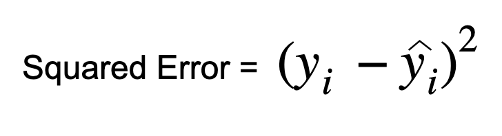
A loss function
A function that calculates loss for the entire data being used is called the cost function.

A cost function
Evaluation Metrics
Mean Absolute Error (MAE)
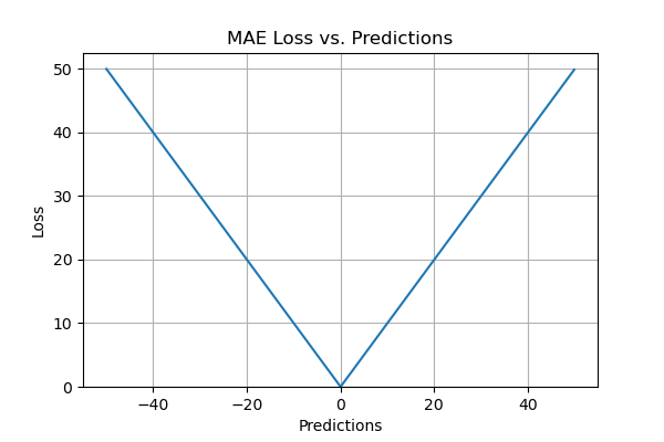
Mean absolute error, also known as L1 loss is one of the simplest loss functions and an easy-to-understand evaluation metric. It is calculated by taking the absolute difference between the predicted values and the actual values and averaging it across the dataset. Mathematically speaking, it is the arithmetic average of absolute errors. MAE measures only the magnitude of the errors and doesn’t concern itself with their direction. The lower the MAE, the higher the accuracy of a model.
Mathematically, MAE can be expressed as follows,

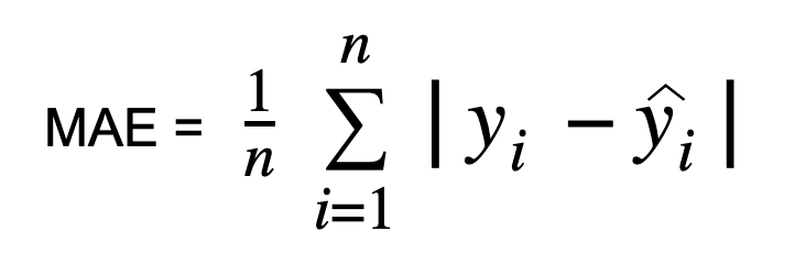
where y_i = actual value, y_hat_i = predicted value, n = sample size
def mean_absolute_error(true, pred):
    abs_error = np.abs(true - pred)
    sum_abs_error = np.sum(abs_error)
    mae_loss = sum_abs_error / true.size
    return mae_loss

Pros of the Evaluation Metric:
- It is an easy to calculate evaluation metric.
- All the errors are weighted on the same scale since absolute values are taken.
- It is useful if the training data has outliers as MAE does not penalize high errors caused by outliers.
- It provides an even measure of how well the model is performing.
Cons of the evaluation metric:
- Sometimes the large errors coming from the outliers end up being treated as the same as low errors.
- MAE follows a scale-dependent accuracy measure where it uses the same scale as the data being measured. Hence it cannot be used to compare series’ using different measures.
- One of the main disadvantages of MAE is that it is not differentiable at zero. Many optimization algorithms tend to use differentiation to find the optimum value for parameters in the evaluation metric.
- It can be challenging to compute gradients in MAE.
Mean Bias Error (MBE)
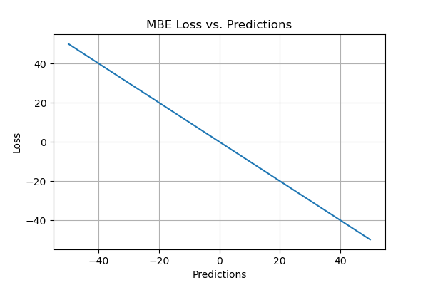
Bias in “Mean Bias Error” is the tendency of a measurement process to overestimate or underestimate the value of a parameter. Bias has only one direction, which can be either positive or negative. A positive bias means the error from the data is overestimated and a negative bias means the error is underestimated. Mean Bias Error (MBE) is the mean of the difference between the predicted values and the actual values. This evaluation metric quantifies the overall bias and captures the average bias in the prediction. It is almost similar to MAE, the only difference being the absolute value is not taken here. This evaluation metric should be handled carefully as the positive and negative errors can cancel each other out.
The formula for MBE,

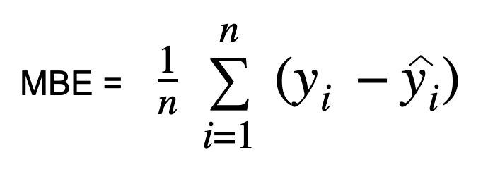
def mean_bias_error(true, pred):
    bias_error = true - pred
    mbe_loss = np.mean(np.sum(diff) / true.size)
    return mbe_loss
Pros of the Evaluation Metric:
- MBE is a good measure if you want to check the direction of the model (i.e. whether there is a positive or negative bias) and rectify the model bias.
Cons of the evaluation metric:
- It is not a good measure in terms of magnitude as the errors tend to compensate each other.
- It is not highly reliable because sometimes high individual errors produce low MBE.
- As an evaluation metric, it can be consistently wrong in one direction. For example, if you’re trying to predict traffic patterns and it always shows lower traffic than what is actually observed.
Relative Absolute Error (RAE)
Relative absolute error is computed by taking the total absolute error and dividing it by the absolute difference between the mean and the actual value.
RAE is expressed as,

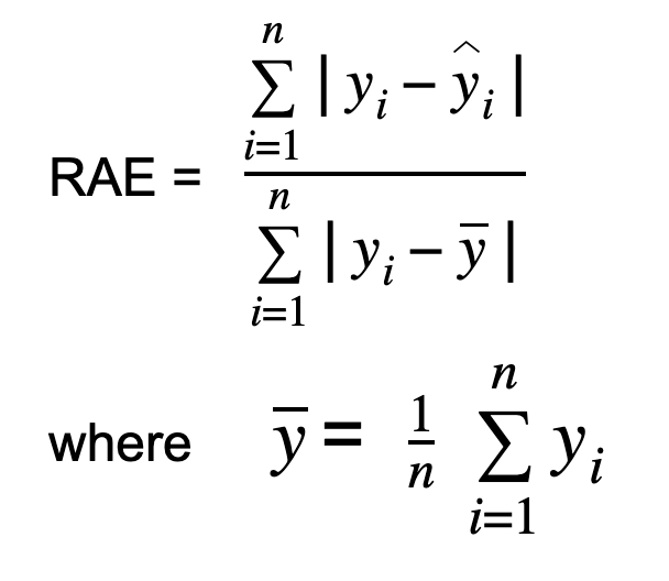
where y_bar is the mean of the n actual values.
RAE measures the performance of a predictive model and is expressed in terms of a ratio. The value of RAE can range from zero to one. A good model will have values close to zero, with zero being the best value. This error shows how the mean residual relates to the mean deviation of the target function from its mean.
def relative_absolute_error(true, pred):
    true_mean = np.mean(true)
    squared_error_num = np.sum(np.abs(true - pred))
    squared_error_den = np.sum(np.abs(true - true_mean))
    rae_loss = squared_error_num / squared_error_den
    return rae_loss
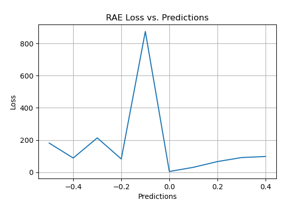
Pros of the Evaluation Metric:
- RAE can be used to compare models where errors are measured in different units.
- In some cases, RAE is reliable as it offers protection from outliers.
Cons of the evaluation metric:
- One main drawback of RAE is that it can be undefined if the reference forecast is equal to the ground truth.
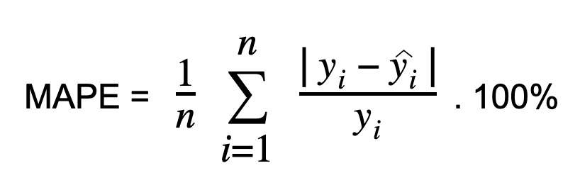
Mean Absolute Percentage Error (MAPE)
Mean absolute percentage error is calculated by taking the difference between the actual value and the predicted value and dividing it by the actual value. An absolute percentage is applied to this value and it is averaged across the dataset. MAPE is also known as Mean Absolute Percentage Deviation (MAPD). It increases linearly with an increase in error. The smaller the MAPE, the better the model performance.

def mean_absolute_percentage_error(true, pred):
    abs_error = (np.abs(true - pred)) / true
    sum_abs_error = np.sum(abs_error)
    mape_loss = (sum_abs_error / true.size) * 100
    return mape_loss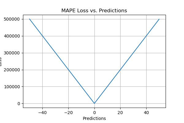
Pros of the Evaluation Metric:
- MAPE is independent of the scale of the variables since its error estimates are in terms of percentage.
- All errors are normalized on a common scale and it is easy to understand.
- As MAPE uses absolute percentage errors, the problem of positive values and the negative values canceling each other out is avoided.
Cons of the evaluation metric:
- One main drawback of MAPE is when the denominator value encounters zero. We are faced with the “division by zero” problem as it is not defined.
- MAPE penalizes negative errors more than positive errors. Hence it is biased when we compare the accuracy of prediction methods as it will pick a method whose values are too low by default.
- Since division operation is used, for the same error a change in the actual value will cause a difference in the loss. Consider a scenario when the actual value is 100 and the predicted value is 75, the loss would be 25%. While the actual value is 50 and the predicted value is 75, the loss would be 50%. But in both cases, the actual error would be the same. i.e., 25.
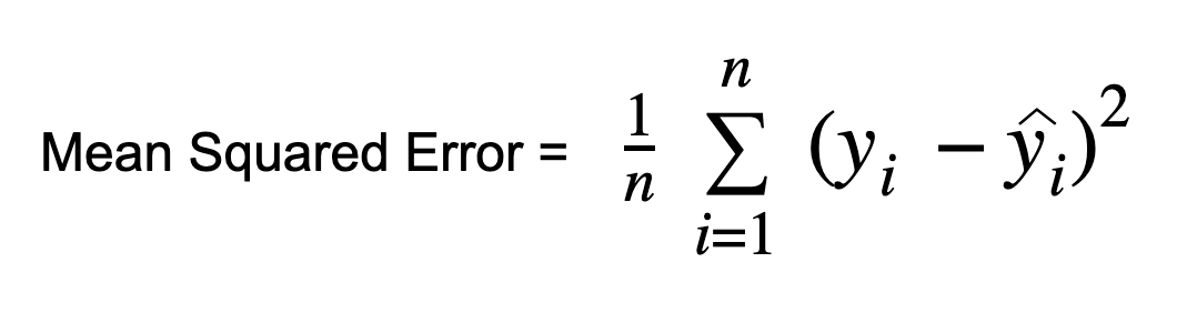
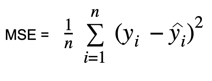
Mean Squared Error (MSE)
MSE is one of the most common regression loss functions. In Mean Squared Error also known as L2 loss, we calculate the error by squaring the difference between the predicted value and actual value and averaging it across the dataset. MSE is also known as Quadratic loss as the penalty is not proportional to the error but to the square of the error. Squaring the error gives higher weight to the outliers, which results in a smooth gradient for small errors. Optimization algorithms benefit from this penalization for large errors as it is helpful in finding the optimum values for parameters. MSE will never be negative since the errors are squared. The value of the error ranges from zero to infinity. MSE increases exponentially with an increase in error. A good model will have an MSE value closer to zero.

def mean_squared_error(true, pred):
    squared_error = np.square(true - pred)
    sum_squared_error = np.sum(squared_error)
    mse_loss = sum_squared_error / true.size
    return mse_loss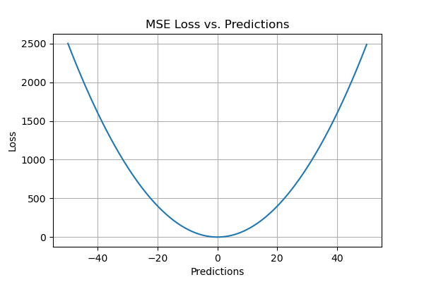
Pros of the Evaluation Metric:
- MSE values are expressed in quadratic equations. Hence when we plot it, we get a gradient descent with only one global minima.
- For small errors, it converges to the minima efficiently. There are no local minima.
- MSE penalizes the model for having huge errors by squaring them.
- It is particularly helpful in weeding out outliers with large errors from the model by putting more weight on them.
Cons of the evaluation metric:
- One of the advantages of MSE becomes a disadvantage when there is a bad prediction. The sensitivity to outliers magnifies the high errors by squaring them.
- MSE will have the same effect for a single large error as too many smaller errors. But mostly we will be looking for a model which performs well enough on an overall level.
- MSE is scale-dependent as its scale depends on the scale of the data. This makes it highly undesirable for comparing different measures.
- When a new outlier is introduced into the data, the model will try to take in the outlier. By doing so it will produce a different line of best fit which may cause the final results to be skewed.
Root Mean Squared Error (RMSE)
RMSE is computed by taking the square root of MSE. RMSE is also called the Root Mean Square Deviation. It measures the average magnitude of the errors and is concerned with the deviations from the actual value. RMSE value with zero indicates that the model has a perfect fit. The lower the RMSE, the better the model and its predictions. A higher RMSE indicates that there is a large deviation from the residual to the ground truth. RMSE can be used with different features as it helps in figuring out if the feature is improving the model’s prediction or not.

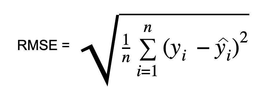
def root_mean_squared_error(true, pred):
    squared_error = np.square(true - pred)
    sum_squared_error = np.sum(squared_error)
    rmse_loss = np.sqrt(sum_squared_error / true.size)
    return rmse_loss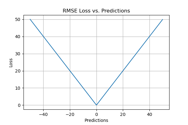
Pros of the Evaluation Metric:
- RMSE is easy to understand.
- It serves as a heuristic for training models.
- It is computationally simple and easily differentiable which many optimization algorithms desire.
- RMSE does not penalize the errors as much as MSE does due to the square root.
Cons of the evaluation metric:
- Like MSE, RMSE is dependent on the scale of the data. It increases in magnitude if the scale of the error increases.
- One major drawback of RMSE is its sensitivity to outliers and the outliers have to be removed for it to function properly.
- RMSE increases with an increase in the size of the test sample. This is an issue when we calculate the results on different test samples.
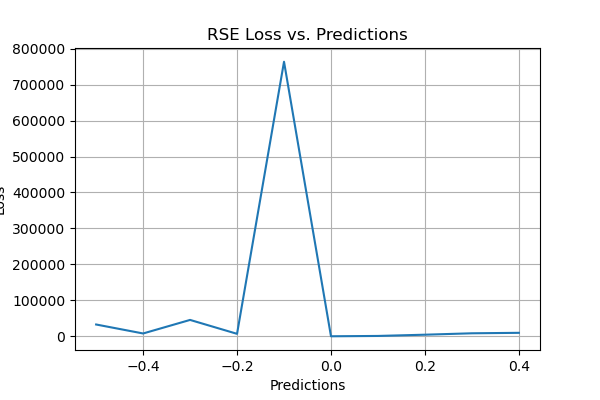
Relative Squared Error (RSE):
In order to calculate Relative Squared Error, you take the Mean Squared Error (MSE) and divide it by the square of the difference between the actual and the mean of the data. In other words, we divide the MSE of our model by the MSE of a model which uses the mean as the predicted value.

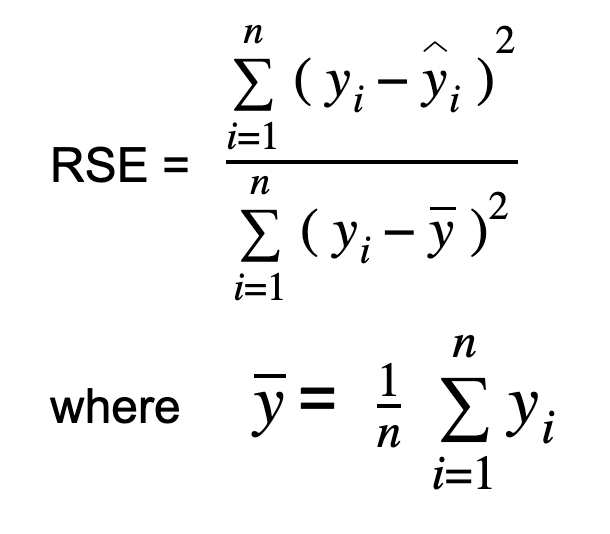
def relative_squared_error(true, pred):
    true_mean = np.mean(true)
    squared_error_num = np.sum(np.square(true - pred))
    squared_error_den = np.sum(np.square(true - true_mean))
    rse_loss = squared_error_num / squared_error_den
    return rse_loss
The output value of RSE is expressed in terms of ratio. It can range from zero to one. A good model should have a value close to zero while a model with a value greater than 1 is not reasonable.
Pros of the Evaluation Metric:
- RSE is not scale-dependent. Hence it can be used to compare between models where errors are measured in different units.
- RSE is not sensitive to the mean and the scale of predictions.
Normalized Root Mean Squared Error (NRMSE)
The Normalized RMSE is generally computed by dividing a scalar value. It can be in different ways like,
- RMSE / maximum value in the series
- RMSE / mean
- RMSE / difference between the maximum and the minimum values (if mean is zero)
- RMSE / standard deviation
- RMSE / interquartile range
# implementation of NRMSE with standard deviation
def normalized_root_mean_squared_error(true, pred):
    squared_error = np.square((true - pred))
    sum_squared_error = np.sum(squared_error)
    rmse = np.sqrt(sum_squared_error / true.size)
    nrmse_loss = rmse/np.std(pred)
    return nrmse_loss
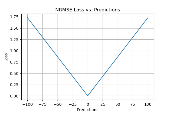
Sometimes choosing the interquartile range may be the best bet as other methods are prone to outliers. NRMSE is a good measure when you want to compare the models of different dependent variables or when the dependent variables are modified (log-transformed or standardized). It overcomes the scale-dependency and eases comparison between models of different scales or even between datasets.
Relative Root Mean Squared Error (RRMSE)
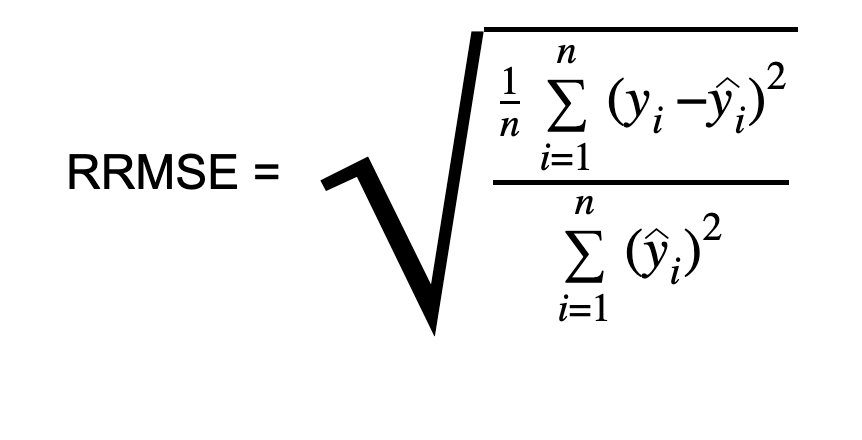
RRMSE is a dimensionless form of RMSE. Relative Root Mean Square Error (RRMSE) is the root mean squared error normalized by the root mean square value where each residual is scaled against the actual value. While RMSE is restricted by the scale of original measurements, RRMSE can be used to compare different measurement techniques. When your predictions are inaccurate, it results in an increased RRMSE. RRMSE expresses the error relatively or in a percentage form. Model accuracy is,
- Excellent when RRMSE < 10%
- Good when RRMSE is between 10% and 20%
- Fair when RRMSE is between 20% and 30%
- Poor when RRMSE > 30%

def relative_root_mean_squared_error(true, pred):
    num = np.sum(np.square(true - pred))
    den = np.sum(np.square(pred))
    squared_error = num/den
    rrmse_loss = np.sqrt(squared_error)
    return rrmse_loss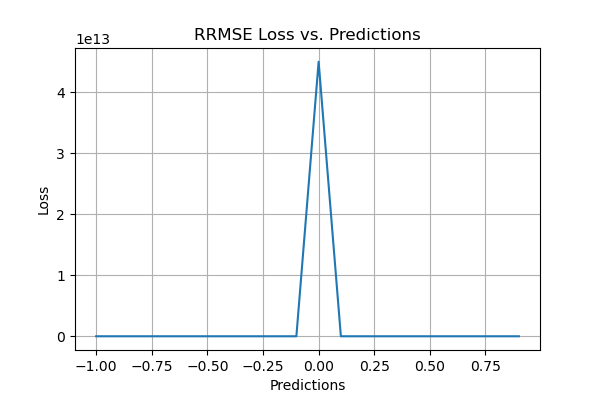
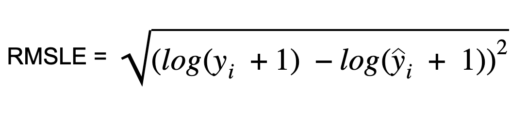
Root Mean Squared Logarithmic Error (RMSLE)
Root Mean Squared Logarithmic Error is calculated by applying log to the actual and the predicted values and then taking their differences. RMSLE is robust to outliers where the small and the large errors are treated evenly.
It penalizes the model more if the predicted value is less than the actual value while the model is less penalized if the predicted value is more than the actual value. It does not penalize high errors due to the log. Hence the model has a large penalty for underestimation than overestimation. This can be helpful in situations where we are not bothered by overestimation but underestimation is not acceptable.

def root_mean_squared_log_error(true, pred):
    square_error = np.square((np.log(true + 1) - np.log(pred + 1)))
    mean_square_log_error = np.mean(square_error)
    rmsle_loss = np.sqrt(mean_square_log_error)
    return rmsle_loss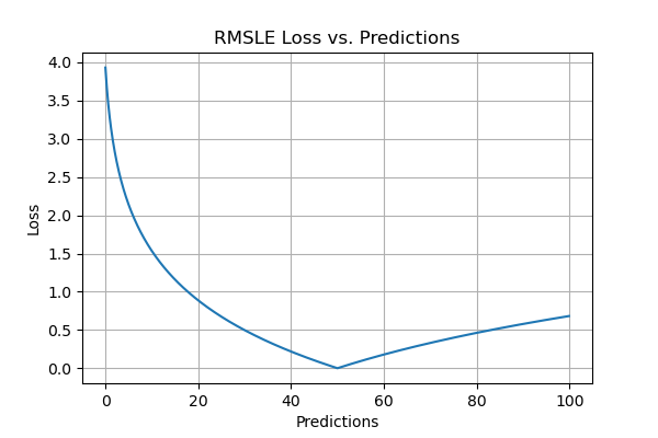
Pros of the Evaluation Metric:
- RMSLE is not scale-dependent and is useful across a range of scales.
- It is not affected by large outliers.
- It considers only the relative error between the actual value and the predicted value.
Cons of the evaluation metric:
- It has a biased penalty where it penalizes underestimation more than overestimation.
Huber Loss
What if you want a function that learns about the outliers as well as ignores them? Well, Huber loss is the one for you. Huber loss is a combination of both linear and quadratic scoring methods. It has a hyperparameter delta (𝛿) which can be tuned according to the data. The loss will be linear (L1 loss) for values above delta and quadratic (L2 loss) for values below it. It balances and combines good properties of both MAE (Mean Absolute Error) and MSE (Mean Squared Error). In other words, for loss values less than delta, MSE will be used and for loss values greater than delta, MAE will be used. The choice of delta (𝛿) is extremely critical because it defines our choice of the outlier. Huber loss reduces the weight we put on outliers for larger loss values by using MAE while for smaller loss values it maintains a quadratic function using MSE.


def huber_loss(true, pred, delta):
    huber_mse = 0.5 * np.square(true - pred)
    huber_mae = delta * (np.abs(true - pred) - 0.5 * (np.square(delta)))
    return np.where(np.abs(true - pred) <= delta, huber_mse, huber_mae)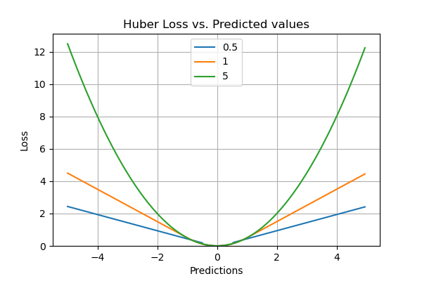
Pros of the Evaluation Metric:
- It is differentiable at zero.
- Outliers are handled properly due to the linearity above delta.
- The hyperparameter, 𝛿 can be tuned to maximize model accuracy.
Cons of the evaluation metric:
- The additional conditionals and comparisons make Huber loss computationally expensive for large datasets.
- In order to maximize model accuracy, 𝛿 needs to be optimized and it is an iterative process.
- It is differentiable only once.
Log Cosh Loss
Log cosh calculates the logarithm of the hyperbolic cosine of the error. This function is smoother than quadratic loss. It works like MSE but is not affected by large prediction errors. It is quite similar to Huber loss in the sense that it is a combination of both linear and quadratic scoring methods.

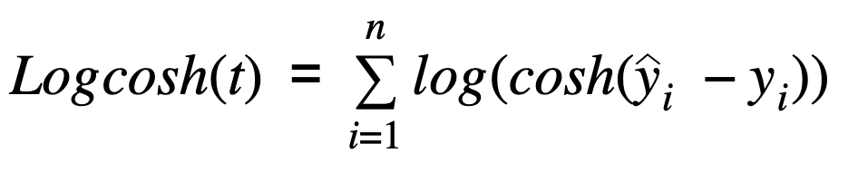
def log_cosh(true, pred):
    logcosh = np.log(np.cosh(pred - true))
    logcosh_loss = np.sum(logcosh)
    return logcosh_loss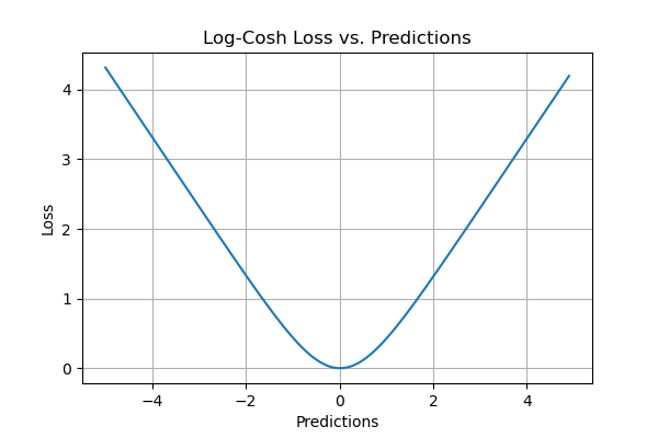
Pros of the Evaluation Metric:
- It has the advantages of Huber loss while being twice differentiable everywhere. Some optimization algorithms like XGBoost favors double differentials over functions like Huber which can be differentiable only once.
- It requires fewer computations than Huber.
Cons of the evaluation metric:
- It is less adaptive as it follows a fixed scale.
- Compared to Huber loss, the derivation is more complex and requires much in-depth study.
Quantile Loss
Quantile regression loss function is applied to predict quantiles. The quantile is the value that determines how many values in the group fall below or above a certain limit. It estimates the conditional median or quantile of the response(dependent) variables across values of the predictor(independent) variables. The loss function is an extension of MAE except for the 50th percentile, where it is MAE. It provides prediction intervals even for residuals with non-constant variance and it does not assume a particular parametric distribution for the response.

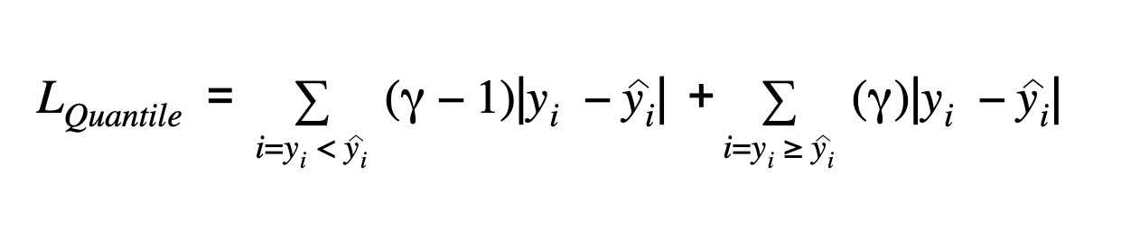
𝛾 represents the required quantile. The quantiles values are selected based on how we want to weigh the positive and the negative errors.
In the loss function above, 𝛾 has a value between 0 and 1. When there is an underestimation, the first part of the formula will dominate and for overestimation, the second part will dominate. The chosen value of quantile(𝛾) gives different penalties for over-prediction and under prediction. When 𝛾 = 0.5, underestimation and overestimation are penalized by the same factor and the median is obtained. When the value of 𝛾 is larger, overestimation is penalized more than underestimation. For example, when 𝛾 = 0.75 the model will penalize overestimation and it will cost three times as much as underestimation. Optimization algorithms based on gradient descent learn from the quantiles instead of the mean.
def quantile_loss(true, pred, gamma):
    val1 = gamma * np.abs(true - pred)
    val2 = (1-gamma) * np.abs(true - pred)
    q_loss = np.where(true >= pred, val1, val2)
    return q_loss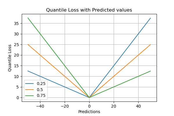
Pros of the Evaluation Metric:
- It is particularly useful when we are predicting an interval instead of point estimates.
- This function can also be used to calculate prediction intervals in neural nets and tree-based models.
- It is robust to outliers.
Cons of the evaluation metric:
- Quantile loss is computationally intensive.
- If we use a squared loss to measure the efficiency or if we are to estimate the mean, then quantile loss will be worse.
Thank you for reading all the way down here! I hope this article was helpful in your learning journey. I would love to hear in the comments about any other loss functions that I have missed. Happy Evaluating!
Connect with me on LinkedIn
References:
- Data Mining Algorithms, Explained using R
- https://www.sciencedirect.com/topics/engineering/mean-bias-error
- https://www.sciencedirect.com/science/article/abs/pii/S1364032115013258
- https://journals.plos.org/plosntds/article?id=10.1371/journal.pntd.0005295
- https://support.sas.com/resources/papers/proceedings17/SAS0525-2017.pdf
- https://stats.stackexchange.com/questions/39002/when-is-quantile-regression-worse-than-ols
Image Credits:
- Cover Image: https://unsplash.com/photos/5fNmWej4tAA
- Graphs and Formulas: All Images by author